Transcript
CHAPTER THREE DENTAL IDENTIFICATION SYSTEM (DIS)
3.1 Overview
It is useful to have a machines can be carried out to patterns recognition quickly and with high perform. For example, the security services that rely on fingerprints as an entry permit, if they depend on humans for the process of checking the fingerprints this take long time If there is an application can do this process quickly and with high accuracy, it will be saving money and time, as well as there are many real life applications that occur in repetitive operations repeatedly and significantly such as reading checks in banks, where the existence of such an application eliminates the requirement that a human perform such a repetitive task.
A neural network system for the dental identification depends on dental radiography images must deals with two basic problems: detection of the features of a dental radiography images and extraction of the essential features of the dental fillings, crowns and bridges and even the missing teeth; and finally the identification.
This chapter explains the research methodology and how has the process of collecting the database and how it was preprocessing. The algorithms that used to resize and compression the images. How it was organized to be feeding to the neural network system. How has the process of training of the neural network system. Testing process also explained in this chapter and the system designed to identify people through the dental radiography images using artificial neural networks approach.
3.2 Dental Identification System Operations
A Neural Network (NN) is to be designed and trained to recognize human through their dental radiography images. Dental identification system (DIS) involves the following series of steps:
Collect anti-mortem (AM) dental records images.
Normalize the AM dental records images.
Train (ANN) using the AM dental images.
Collect the post-mortem (PM) dental records images.
Normalize the PM dental images.
Test (ANN) using the PM images.
3.2.1 Database Collecting
The starting point of working on the system was the collecting of database with all images that would be used for training and testing the system. The images that are used in this work are .jpg format. Using adobe Photoshop software tool, all images were divided into four quarters and of the same size and the same resolution.
The database that was used in this work is made up of dental radiography images which are obtained from the dental clinic in the Department of Dentistry at Near East University. The size of the images are (1600x800) pixel. The original database contains 50 images of the full mouth (upper jaw and lower jaw), representing 50 persons. Figure 3.1 shows an example of these dental radiography images.
Figure 3.1 Example of Dental Radiography Images.
The database was expanded to 150 dental radiography images by adding two types of noise (Grain noise, Gaussian noise) to each image. This presents the neural network with more challenging task, and provides a variety of imaging problem that could occur to original dental radiography images. Figure 3.2 shows an example of original image and its noisy versions.
a. Original Image
b. First Noise (Grain Noise)
c. Second Noise (Gaussian Noise)
Figure 3.2 Example of Original Image and Its Noisy Versions.
Each image in the database was divided into four quarters of equal size (800 x 400) pixels. The reason is to consider that (PM) cases may not have full mouth images. Therefore, the total number of images after segmentation is 600 images.
These images will be used for both training and testing the (DIS). Figure 3.3 shows an example of a segmented full mouth image. The complete database segmented images are available in Appendix I.
Quarter 3.
Quarter 1.
Quarter 4.
Quarter 2.
Figure 3.3 Example of A Segmented Full Mouth Image.
Segmenting the images into four quarters has the advantages of:
Minimizing complexity of the algorithm.
Minimizing memory usage by simulating systems.
Maximizing machine speed.
Improving the performance of IC-based chips; if such systems are implemented on ICs (using microcontrollers).
Reduces the cost associated with commercializing such a system.
3.2.2 Preprocessing
The preprocessing stage in dental identification system is a very important stage. The full dental radiography images were resized to (800 x 400). The dimension of the dental radiograph images must be the same to make the feature extraction process easier.
3.2.2.1 Image Normalization
Normalization is mapping the range of the pixels values to a suitable range for subsequent processing. Usually, this is achieved by a normalization transform that maps the ‘black’ gray scale to ‘0’ and the ‘white’ gray scale to ‘1’. The simplest normalization transform is a division by 255, which is a linear transform that will maintains constant spacing between gray scales after transformation. We can represent the normalization operation with the equation:
(3.1)
We utilize image compression in order to reduce the complexity of the neural network, and hence cut down the computational cost particularly during the training phase.
3.2.2.2 Image Compression
The task of compression is to transform the input normalized images array to a reduced size array for the same images Thus; the compression step is effectively performing function.
The compression operation that used for resize the images was down sampling method, this method depends on the down sampling factor that determines the down sampling value, for example if the down sampling factor was equal to 4 then the images size will be 1/4 of the original image. The down sampling method based on the value of the down sampling factor. Where down sampling factor determines the number of pixels that are left and taken from the original image. As in the above example, the down sampling factor is equal to 4 this means that will be taking one pixel of every 4 pixels, which takes one pixel and leaves the following three in successions to the end of the entire image matrix as shown in figure below.
Figure 3.4 Down Sampling Process.
Table 3.1 Down Sampling Compression Process.
Dental X-Ray Images
Dental Image Size
Down Sampling Parameter = 4
Down Sampling Parameter = 5
Quarter 1.
800 x 400 = 320000
200 x 100 = 20000
160 x 80 = 12800
Quarter 2.
800 x 400 = 320000
200 x 100 = 20000
160 x 80 = 12800
Quarter 3.
800 x 400 = 320000
200 x 100 = 20000
160 x 80 = 12800
Quarter 4.
800 x 400 = 320000
200 x 100 = 20000
160 x 80 = 12800
Total = 1280000
Total = 80000
Total = 51200
The size of dental images is very large to work on the system. The large number of the inputs means longer time in processing stage. To reduce the processing time, we must reduce the input size. We can make this operation by using averaging process.
The reduced matrices of the pixel values are calculated from a weighted average of pixels in the nearest neighborhood as shown in Figure 3.5. Depending on the averaging mask parameter that we decided in the program represented by (a*b), this parameters represent the vertical and horizontal neighborhood of the pixel. The output matrices dimension after interpolation process will be 1/a*b of the input matrices. For example, if we have the matrix 12x15 and the averaging mask parameter are 3*3 then the input matrices will be after averaging 4x5 as shown in figure 3.5.
Figure 3.5 Averaging Process.
Table 3.2.a Averaging Resize Process with Down Sampling Value = 4
Dental X-Ray Images
Down Sampling Parameter = 4
Averaging Mask
2 x 2 = 4
Averaging Mask
4 x 4 = 16
Quarter 1.
200 x 100 = 20000
100 x 50 = 5000
50 x 25 = 1250
Quarter 2.
200 x 100 = 20000
100 x 50 = 5000
50 x 25 = 1250
Quarter 3.
200 x 100 = 20000
100 x 50 = 5000
50 x 25 = 1250
Quarter 4.
200 x 100 = 20000
100 x 50 = 5000
50 x 25 = 1250
Total = 80000
Total = 20000
Total = 5000
Table 3.2.b Averaging Resize Process with Down Sampling Value = 5
Dental X-Ray Images
Down Sampling Parameter = 5
Averaging Mask
2 x 2 = 4
Averaging Mask
4 x 4 = 16
Quarter 1.
160 x 80 = 12800
80 x 40 = 3200
40 x 20 = 800
Quarter 2.
160 x 80 = 12800
80 x 40 = 3200
40 x 20 = 800
Quarter 3.
160 x 80 = 12800
80 x 40 = 3200
40 x 20 = 800
Quarter 4.
160 x 80 = 12800
80 x 40 = 3200
40 x 20 = 800
Total = 51200
Total = 12800
Total = 3200
Figure 3.6 shows the size of the original image after down sampling with the different parameters.
a. Original Image
Image Size = 1600 x 800
Down Sampling by 2 Pixels
Image Size = 800 x 400
Down Sampling by 4 pixels
Image Size = 400 x 200
Down Sampling by 5 Pixels
Image Size = 320 x 160
Averaging Mask = 4 x 4
Down Sampling Value by 4 Pixels
Image Size = 5000
Averaging Mask = 2 x 2
Down Sampling Value by 5 Pixels
Image Size = 12800
Figure 3.6 Image Compression Using Down Sampling and Averaging Process.
3.2.2.3 Image Reading
A digital image is composed of pixels which can be thought of as small dots on the screen. A digital image is an instruction of how to color each pixel.
Gray scale image is the image we will mostly work with in this system. It represents an image as a matrix where every element has a value corresponding to how bright/dark the pixel at the corresponding position should be colored. There are two ways to represent the number that represents the brightness of the pixel: The double class (or data type), this assigns a floating number ("a number with decimals") between 0 and 1 to each pixel. The value 0 corresponds to black and the value 1 corresponds to white. The other class is called uint8 which assigns an integer between 0 and 255 to represent the brightness of a pixel. The value 0 corresponds to black and 255 to white. The class uint8 only requires roughly 1/8 of the storage compared to the class double. On the other hand, many mathematical functions can only be applied to the double class.
Through what previously mentioned above from normalize paragraph, the images that used in order to train and test the dental identification system are grayscale double images.
3.2.2.4 Image Vectorization
A vector is defined by placing a sequence of numbers within square braces. Matlab is a software package that makes it easier to enter matrices and vectors, and manipulate them. To prepare the training set patterns to be fed in to the neural network must be arranged to input matrix, this process is called vectorization.
The dimension of the vector matrix for the 50 person it will be different depend on the experiment that carried out and depending on the values ??and averaging and down sampling parameters that used in the experiment.
3.3 Using Matlab
Matlab is a simple and useful high-level language for matrix manipulation. Since images are matrices of numbers, many vision algorithms are naturally implemented in Matlab. It is often convenient to use Matlab even for programs for which this language is not the ideal choice in terms of data structures and constructs.
In fact, Matlab is an interpreted language, which makes program development very easy, and includes extensive tools for displaying matrices and functions, printing them into several different formats like Postscript, debugging, and creating graphical user interfaces. In addition, the Matlab package provides a huge amount of predefined functions. Matlab has an artificial neural networks toolbox, through this toolbox we can programming and design the system in ease way.
3.4 Implementation of the Neural Network
There are a few issue that have to be taken into consideration before the implementing the neural network. The following subtopics will be discussed.
3.4.1 Define BPNN Architecture and Design
Back propagation network architecture involves the selecting of an appropriate number of layers and the number of nodes in each layer based on the size and type of the application and the problem involved. As stated earlier, the neural network architecture consists of three layers, which are the input layer, hidden layer and also the output layer. The required number of nodes in each layer also differs from each dataset based on the classification problem. Thus, the number of nodes in the input and output layers are determined by the input and output variables based on the dataset.
Nevertheless, the essentials number of hidden nodes did not present. These hidden nodes are required for the computing difficult functions recognized as the non-separable functions. The number of nodes in the hidden layer determines the network’s learning capabilities. It’s been crucial of selecting the appropriate number of hidden layer for the optimal network design. The hidden layer size may affect the complexity and the required time for training but, out of all, it could influence its competence to generalize. However, there is no an appropriate standard rule or theory to determine the optimal number of hidden nodes.
3.4.2 Formulation of Weight Adjustment
The main focus in weight adjustment process is the activation function. The conventional sigmoid function will be applied to the standard backpropagation.
3.4.3 Define the Learning Rate and Momentum Factor
The core parameters for neural networks are the learning rate and momentum factor, as these values will have an effect on the learning performance.
3.4.4 Define the Maximum Error
Maximum error is another parameter that should be taken into the consideration. This maximum error should be the stopping criteria for the backpropagation training. As for this system, the maximum error is set different values. Besides that, the training process of the backpropagation is been set to a maximum of 20,000 iterations, or until the error reaches the maximum error. It is adequate for the network to train the dataset within 20,000 iterations and converge to the solution. Since the main focus of this system is the faster convergence rate, thus the minimum iteration is important.
3.5 Training Using Back Propagation
An interesting aspect of Back Propagation Neural Networks (BPNN) in the Multi-Layer Perceptron (MLP) is that during the learning process, the hidden layers build an internal representation of the inputs that are useful to produce the output.
The adjustment of neural network parameters using back propagating of observed error at the network output is the most famous technique for supervised training of neural networks. Back Propagation depends on a sophisticated system of training contains a layers of neurons, begin with the first input layer which received the value according to their sequence in from the images vector matrix, followed by one or more of hidden layers of then the output layer.
The size of the input layer must be identical to the size of the image pixels and the size of output layer must be equal to the number of the persons that take their dental radiographs to be trained in this case the output layer was equal to 50.
A series of experiments have been carried out with different number of training and testing images and different values of the training parameters as shown in tables in the next chapter. The value of learning rate and momentum factor for each experiment has been chosen from different values as shown in table 3.3.
Table 3.3 Values of Learning Rate and Momentum Factor.
Experiment Number
Learning Rate Values
Momentum Factor Values
1st Experiment
0.005
0.3
2nd Experiment
0.00053
0.021
3rd Experiment
0.3
0.004
4th Experiment
0.003
0.7
5th Experiment
0.08
0.6
6th Experiment
0.00053
0.021
7th Experiment
0.003
0.6
8th Experiment
0.001
0.2
Figure 3.7 shows the neural network design of dental identification system:
285750124460O1
O2
O50
X1
X2
X3
X4
Xi
H1
H2
H3
Hj
00O1
O2
O50
X1
X2
X3
X4
Xi
H1
H2
H3
Hj
Figure 3.7 Neural Network Design.
Figure 3.8 shows the block diagram of the dental identification system, represented the three stage of the system. Starting with database collection, which is obtained from dental clinic in department of dentistry at Near East University. The second stage was to pre-processing these images to prepare it to the neural network stage. The preprocessing stage include adding noise to the images to extended the database images number and normalizing the pixel value and compression with down sampling and averaging processes to make the images in reduced size. The neural network stage involved training and testing processes. The training process was carried out using training set form database; the testing process was carried out using different images set equipped to the testing process.
045720Calculating dental radiography images
Image normalization
Preprocessing stage
Adding noise
Image compression
Database collecting stage
ANN stage
Training ANN with the training image
The trained ANN
Training
Testing images
Testing
Output
Image vectorazing
00Calculating dental radiography images
Image normalization
Preprocessing stage
Adding noise
Image compression
Database collecting stage
ANN stage
Training ANN with the training image
The trained ANN
Training
Testing images
Testing
Output
Image vectorazing
Figure 3.8 Block Diagram of DIS.
933450-148590Set Random Hidden and Output Weights
Calculate MSE
Input Vector Matrix
Training Part
Back Propagation Algorithm
Calculate the Output for Each Pattern
If
MSE > Error Goal
No
Finish Training
Yes
Start
Calculate MSE
Reading Images and Neural Network Parameters
Save the Last Weights
Display the MSE and Number of Iteration
00Set Random Hidden and Output Weights
Calculate MSE
Input Vector Matrix
Training Part
Back Propagation Algorithm
Calculate the Output for Each Pattern
If
MSE > Error Goal
No
Finish Training
Yes
Start
Calculate MSE
Reading Images and Neural Network Parameters
Save the Last Weights
Display the MSE and Number of Iteration
Figure 3.9 Flow Chart Diagram of the System (Training Process).
-396240-2800351600 x 800
800 x 400
800 x 400
800 x 400
800 x 400
50 x 25
50 x 25
50 x 25
50 x 25
X1
X2
X3
X1250
H1
H2
Hj
O1
O2
O50
Person 50
Person 2
Person 1
Original Image
Four Quarters of the Original Image
Compressed Quarter Images
Input Layer with 1250 Input Neurons
Hidden Layer with j Hidden Neurons
Output Layer with 50 Output Neurons
001600 x 800
800 x 400
800 x 400
800 x 400
800 x 400
50 x 25
50 x 25
50 x 25
50 x 25
X1
X2
X3
X1250
H1
H2
Hj
O1
O2
O50
Person 50
Person 2
Person 1
Original Image
Four Quarters of the Original Image
Compressed Quarter Images
Input Layer with 1250 Input Neurons
Hidden Layer with j Hidden Neurons
Output Layer with 50 Output Neurons
Figure 3.10 Dental Identification System Design (First Experiment).
-243840-4495801600 x 800
800 x 400
800 x 400
800 x 400
800 x 400
80 x 40
80 x 40
80 x 40
80 x 40
X1
X2
X3
X3200
H1
H2
Hj
O1
O2
O50
Person 50
Person 2
Person 1
Original Image
Four Quarters of the Original Image
Compressed Quarter Images
Input Layer with 3200 Input Neurons
Hidden Layer with j Hidden Neurons
Output Layer with 50 Output Neurons
001600 x 800
800 x 400
800 x 400
800 x 400
800 x 400
80 x 40
80 x 40
80 x 40
80 x 40
X1
X2
X3
X3200
H1
H2
Hj
O1
O2
O50
Person 50
Person 2
Person 1
Original Image
Four Quarters of the Original Image
Compressed Quarter Images
Input Layer with 3200 Input Neurons
Hidden Layer with j Hidden Neurons
Output Layer with 50 Output Neurons
Figure 3.11 Dental Identification System Design (Second Experiment).
3.6 Testing DIS
After training is completed, in order to test the performance of the dental identification system, the testing process carried out by using a different set of dental
X-ray images of the same persons that used their X-ray images for the training process, by adding one type of noise to the images to make it different from the original dental radiography images. Figure 3.12 shows an example of testing image for the one person.
Figure 3.12 Example of Testing Image.
2232660204470Start
00Start
1676400194945Reading Images
00Reading Images
27108151397000
271081510287000
2530475-545465Input Vector Matrix
00Input Vector Matrix
272224513462000
2546985-486410Feed Forward Pass
00Feed Forward Pass
271462513271500
2499360-381635Calculate Outputs
00Calculate Outputs
270129021463000
2517140-436245Save Output Values
00Save Output Values
268605021590000
2085975159385Finish Testing
00Finish Testing
Figure 3.13 Flow Chart Diagram of the System (Testing Process).
3.7 Summary
This chapter discusses the methodology of the dental identification system (DIS) in detail. Database collecting, normalized, algorithms that used to resize and compression the images. How it was organized to be feeding to the neural network system, and training and testing the system. Next chapter will contain the results that obtained from the training and testing the dental identification system.