Transcript
Ryerson University
Department of Chemical Engineering
CHE 415 Unit Operations II
Lab Report
Experiment #2: Vapor-Liquid Equilibrium
_______________________________________________
Experiment Performed on: October 5, 2006
Report Submitted to
Dr.
By Group # 1 Section # 021 1. (Inspector)
2. (Data Reporter)
3. (Leader)
Date Report Submitted: October 12, 2006.
Marking Scheme
Formatting Answer to all 6 questions in each Report Section / 10
General Appearance; Grammar and Spelling / 5
Complete and Informative Tables and Graphs / 15
Contents Accuracy and Precision of Results / 20
Comparison with Literature Data / 10
Influence of Procedural Design on Results / 10
Logic of Arguments / 20
Sample Calculations / 10
_____
Total: / 100
Table of Contents
Introduction 3
THEORETICAL BACKGROUND 4
Technical procedure 6
Results and discussion 8
Error Analysys 11
Conclusion and recommendations 13
REFERENCES 14
APPENDIX
RAW DATA 15
Sample Calculations 15
List of Figures
Figure 1: VLE Plot for Methanol-Water System 5
Figure 2: Othmer Still Apparatus 7
Figure 3: Table of found densities and weight percentages 8
Figure 4: Table of obtained experimental data 8
Figure 5: Table of theoretical mole fractions using Raoult’s law 9
Figure 6: Phase diagram for methanol-water system 9
Figure 7: x-y diagram for methanol-water system 10
Figure 8: Percent Error for Liquid-Vapor Equilibrium Mole Fractions 11
Figure 9: Distillate Data for Determination of Density 15
Figure 10: Pot Liquid Data for Determination of Density 15
INTRODUCTION
This experiment was designed to determine if the experimental vapor-liquid equilibrium of a methanol and water solution acted as an ideal solution. This was proven by calculating theoretical ideal equilibrium values using Raoult’s Law. Once these theoretical values were determined, they were compared to the experimental data, which was calculated using Antoine’s equation.
The experiment was preformed using an Othmer still apparatus. This experimental design theoretically predicts the exact equilibrium concentrations of a binary mixture between its liquid and vapor phases. In order to achieve a liquid-vapor equilibrium trend, a few trials must be run with this apparatus. It was possible to perform three trials within the time limitations.
After comparison of the results, it was concluded that this mixture was not acting as an ideal solution. The percent errors, comparing experimental mole fractions to theoretical values, all exceeded 25% in both liquid and vapor phases. Some values were determined with such great error that the percentage error exceeded 1000%. To say the least, this experiment did not perform as planned. Many errors were encountered with outcomes which were not expected.
Theoretical Background
Vapor-liquid equilibrium (VLE) data is very important in the design of separation processes in the chemical industry. When the system is ideal, it is fairly simple to estimate the vapor-liquid equilibrium. In this experiment, the vapor-liquid equilibrium relationship of a binary system, a methanol and water solution, will be examined.
The vapor pressure and the composition in equilibrium with a solution can be used to describe the thermodynamic properties of the liquids that compose a solution. Raoult’s law is used to relate the vapor pressure of the components in a solution to their composition. The law assumes ideal behavior and is given by
yAP = xAPA(T) (1)
where PA is the vapor pressure of pure component A at the equilibrium temperature and P is the equilibrium pressure. This equation illustrates that the vapor pressure of each component in a solution depends on the vapor pressure and the mole fraction of the individual component.
Since it is desired to find PA in Raoult’s law in order to solve for the mole fractions, Antoine’s equation can be used. This equation is a relationship between temperature and vapor pressure of liquids
log10P = A – B /(T + C) P (mm Hg), T (C) (2)
where A, B and C are the Antoine coefficients that vary from substance to substance, T is absolute temperature and P is vapor pressure.
Methanol-water solutions are said to be non-ideal but Raoult’s law can still be applied to this mixture. Mixtures which are considered to be non-ideal have a common phenomenon and are referred to as azeotropes. This is the point on the vapor-equilibrium curve which produces a minimum or maximum for the generated data. The vapor-liquid equilibrium curve for the methanol-water system does not display this kind of trend, as seen in the theoretical VLE graph for the methanol-water system, taken from Perry’s Chemical Engineering Handbook,
Figure 1: VLE Plot for Methanol-Water System
This information should not be overlooked, especially since the main goal of this experiment was to determine if the methanol-water mixture would behave as an ideal solution.
TECHNICAL PROCEDURE
The Othmer still apparatus was used in this experiment. Glassware was cleaned and an initial solution of 50% methanol and 50% water, by volume, was used in the Othmer still apparatus. The boiling pot was filled with the 50/50% solution, where there were already boiling chips placed inside of it. The gas to the bunson burner was turned on as well as the burner itself, where a flame was produced in order to heat up the liquid. Heat control was observed in order to prevent escaping vapors from the apparatus. The condensing vapors were not allowed to exceed the top section of the condensing column.
A thermometer was inserted into the boiling pot before beginning the experiment. This was in order to monitor the temperature, which should remain constant once it is in equilibrium. The solution was left to achieve an equilibrium point, after it was determined that the temperature would no longer fluctuate. This temperature was recorded for raw data. The heat source was removed and the system was let to cool down. To speed up cool down time of the liquid in the distillate and the liquid of the boiling pot, both were removed by placing them into clean flasks or beakers and they were then placed into a cold water bath.
After the liquids were cooled, they were both placed into pre-weighed pyncometers to be weighed. By doing this, densities could be determined for both liquids. For the reason of comparison to theoretical references, cool down temperatures were determined by corresponding them to temperatures referenced with densities of theoretical values. The liquids were then disposed of in waste containers and glassware was cleaned.
This entire procedure was then repeated for a 28.5/71.5 % volume mixture and a 10/90 % volume mixture of methanol to water. All data was recorded as mentioned above. Once the trials were completed, all glassware was washed and put away and the apparatus was cleaned.
Figure 2: Othmer Still Apparatus
Results and Discussion
Three solutions of 0.50, 0.285 and 0.10 mole fraction of methanol were prepared and were allowed to reach equilibrium within the Othmer Still. The corresponding boiling temperatures found for the three solutions were 66oC, 68oC and 87oC, respectively. Upon completion of this experiment the mole fractions of the distillate and the remaining pot liquid were determined. This was accomplished by measuring the densities of both liquids and finding the corresponding weight percent in the mixture from a reliable source. The following were the calculated densities and weight percentage,
Temperature ( C) Distillate Pot Liquid
Density (g/mL) weight % Density (g/mL) weight %
66 0.8444 81 0.9132 51
68 0.8832 65 0.9672 19.5
87 0.9372 40 0.986 8
Figure 3: Table of found densities and weight percentages
The weight percent was then divided by the molecular weight of the corresponding material to find the number of moles, and mole fraction was then found. The results were as follows,
Temperature ( C) Mole Fraction (Liquid) Mole Fraction (Vapour)
CH3OH H20 CH3OH H20
66 0.3693 0.6307 0.7057 0.2943
68 0.1199 0.8801 0.5109 0.4891
87 0.0466 0.9534 0.2727 0.7273
Figure 4: Table of obtained experimental data
As can be seen from the experimental data, as the initial mole fraction of methanol decreased, the boiling point temperature increased and approached that of pure water at 1000C. The values of vapour liquid equilibrium were compared to the values that Raoult’s law produced at the same temperatures to determine if the solution could be considered ideal. The values calculated using Raoult’s law were as follows,
Temperature (oC) Mole Fraction (Liquid) Mole Fraction (Vapour)
CH3OH H20 CH3OH H20
66 0.9371 0.0629 0.9838 0.0162
68 0.8430 0.1570 0.9557 0.0442
87 0.2357 0.7643 0.5286 0.4714
Figure 5: Table of theoretical mole fractions using Raoult’s law
It can be seen that the values from Raoult’s law and the values determined experimentally did not seem to coincide. This is most likely do to the fact that the system was not given enough time to reach equilibrium. This can be proven if a plot of the phase diagram is examined with the experimental and, Raoult’s law data added will show if equilibrium was actually reached. The plot is as follows,
Figure 6: Phase diagram for methanol-water system
It can be seen that the experimental values did not exhibit the same behaviour nor did they fall within the reliable data range. This suggest that the system did not reach equilibrium before the distillate sample was collected. The Raoult’s law calculated values did lie within or close to the acceptable data range, though. This showed that Raoult’s law calculated values preformed better than the laboratory values did.
In Figure 7, the theoretical plot for the vapour-liquid equilibrium trend for the methanol-water solution was plotted, from a reliable source, as well as the experimental trends and the Raoult’s law trend. It can be seen that the experimental data followed the theoretical trend very closely, which would suggest that this methanol-water solution could follow an ideal trend in relation to its theoretical set point. The Raoult’s law values remained near the end of the theoretical trend line and did not display the curve. Perhaps this shows that Raoult’s law values disproves methanol-water systems as ideal solutions. It did seem though that the error lied with Raoult’s law values and not with the experimental trend.
Figure 7: x-y diagram for methanol-water system
ERROR ANALYSIS
The main error found in this experiment was the failure to achieve equilibrium between the vapor and the liquid. From the results presented, it was obvious that not enough time was elapsed in order for equilibrium to occur, even though the final temperatures were steady and constant for a long enough time. Because the equilibrium was not achieved, the calculations for Raoult’s law did not hold and a major percentage error was found for all three trial runs. The errors are described below.
Percent Error
Liquid Vapour
CH3OH H20 CH3OH H20
60.6 535.2 28.3 1713.7
85.8 249.1 46.5 1005.2
80.2 29.6 48.4 54.3
Figure 8: Percent Error for Liquid-Vapor Equilibrium Mole Fractions
Since these error values were so high, this could be proving that the methanol-water system is absolutely not an ideal solution. But often in literature used for examples, methanol-water systems are assumed to be ideal. These grossly large errors show that the assumption should never be made and that water and methanol do not behave ideally. Note, though, that the VLE graph for methanol-water systems do not produce an azeotrope.
It was also observed that the second trial had a temperature that was very close to the first trial. This meant that the thermometer was not inserted properly. It is known this was an error because at varied concentration solutions, the equilibrium temperature will change. So, not only was the second trial not run long enough, but the first might have been as well. From the percentage error, it was seen that incorrect temperature readings also accounted for a major disfunction in this experiment. These calculated error percentages show that the third trial ran more smoothly than the first two. This was most likely because the last trial was the point of realization of the thermometer was not inserted properly, and was then fitted properly into the boil pot.
The receiver where distillate was collected was leaking as well. Distillate was being lost when it should have been staying in the receiver and flooding over back into the boiling pot.
Time constraints were also a problem for this experiment. In order to perform the presented objectives, a longer time period would be necessary. Time was the most important variable for this experiment and therefore, the more of it supplied, the more room for improvement. If these trials were ran with longer equilibrium times, that is, longer times to make sure equilibrium was reached, the solution may have reached close to an ideal solution. Perhaps if the percentage errors were between 15% to 20%, then the solution may have been deemed almost ideal. Also, if the percentage errors themselves, which were presented in Figure 7, were close relative to each other or following a trend, then perhaps the experiment would have not been as dysfunctional as it was.
CONCLUSION AND RECOMMENDATIONS
This experiment was preformed in order to determine if the methanol and water solution behaved as an ideal solution by determining the liquid-vapor equilibrium of the mixture. From the results found, it was seen that this mixture did not act as an ideal solution. The percentage errors between the experimental solution and the theoretical solution were found to be very large. This experiment showed that the solution did not act ideally because of the tremendous error found.
The major source of error for this experiment was the lack of time spent for reaching a sound liquid-vapor equilibrium. It is believed that if there was more time allowed for the laboratory experiment, proper liquid-vapor equilibrium values would have been obtained.
REFERENCES
1. Benitez, Jaime, Principles and Modern Applications of Mass Transfer Operations, John Wiley & Sons Inc., New York, 2002
2. Perry, H.H., and D. Green, Perry’s Chemical Engineers’ Handbook, 6th Ed., McGraw-Hill Inc., New York, 1984.
3. Winnick, Jack, Chemical Engineering Thermodynamics, John Wiley & Sons, New York, 1997. (pg. 560-561)
4. _http://antoine.frostburg.edu/chem/senese/101/liquids/glossary.shtml_
5. http://www.tannerm.com/raoult.htm
APPENDIX
Raw Data
DISTILLATE
Temperature (°C) Mass of Pycnometer (g) Mass of pycnometer and solution (g) Volume (ml)
66 12.89 34 25
68 12.74 34.82 25
87 12.76 36.19 25
Figure 9: Distillate Data for Determination of Density
POT LIQUID
Temperature (°C) Mass of Pycnometer (g) Mass of pycnometer and solution (g) Volume (ml)
66 12.94 35.77 25
68 12.82 37 25
87 12.77 37.42 25
Figure 10: Pot Liquid Data for Determination of Density
Sample Calculations
Using a 50/50% volume solution of methanol:
Moles of methanol = (175 ml)*(0.791 g/mL)/ 32 g/mol = 4.33 moles
Moles of water = (175 ml)*(0.995 g/mL) / 18 kg/mole = 9.67 moles
Total Moles: 4.33 + 9.67 = 14 moles
Methanol: 4.33 / 14 = 0.31 mole fraction
Water: 9.67 / 14 = 0.69 mole fraction
Finding mole fractions of vapour condensate and pot liquid using first run data:
(Mass of pycnometer + condensate - Mass of empty pycnometer) / volume of pycnometer
= (12.89 g - 34 g) / 25 mL
= 0.8444 g/mL
From Table 3-109 (Densities of Aqueous Organics Solutions) in Perry’s Handbook for Methyl Alcohol at 20°C, 0.8444 g/cm3 corresponds to 81 %wt solution of methanol. If we assume a 1 gram solution, then 0.81 grams will be methanol and 0.19 grams water.
Then,
Moles of methanol = 0.81 g / 32g/mol = 0.0253 moles
Moles of water = 0.34 g / 18 g/mol = 0.01056 moles
Total moles = 0.0253 + 0.01056 = 0.03586
Methanol mole fraction in distillate: 0.0253/ 0.03586 = 0.7055 mole fraction
Water mole fraction in distillate: 0.01056 / 0.03586 = 0.2945 mole fraction
Finding vapour pressure to use in Raoult’s law:
Using Antoine’s equation1
log10P* = A – B /(T + C) [1] P* (mm Hg), T (C)
with:
Range (C) A B C
Methanol: 64 to 110 7.87863 1473.11 230
Water: 60 to 150 7.96681 1668.21 228.0
At a boiling point of 66C at 1 atmosphere
Methanol: log10P* = 7.87863 - (1473.11/(66+230))= 2.902
P* = 797.824 mmHg
Water: log10P* = 7.96681 – 1668.21 / (66 + 228.0) = 2.293
P* = 196.17 mmHg
Finding mole fractions of vapour and liquid:
Raoult’s law in terms of pressure
xmethanol = (Ptotal – P*Water) / (P*Methanol – P*Water) [2A]
= (760 – 196.17) / (797.824 – 196.17)
= 0.9371
xwater = 1.0 – 0.9371
= 0.063
ymethanol = (P*Methanol)*(xmethanol / Ptotal) [2B]
= 797.824 * (0.9371/760)
= 0.984
ywater = 1.0 – 0.984
= 0.016
17