Simpson's Rule: Enhancing area approximation using parabolas

Simpson's rule is a widely used numerical integration technique that was originally documented by Thomas Simpson, an English weaver who self-taught himself mathematics in the 18^th century (Schwartz, 2011). Since the basis of this method involves using parabolas to approximate the shape of a curve, to generate any parabola, three consecutive points are required. Thus, to correctly apply this method, three or more odd equally spaced consecutive data points are needed along a curve. To obtain an odd number of data points along a curve, an even number of subintervals, \(n\), must be used \((n≥2)\) – a subinterval is the space between two points. In fact, for every two subintervals, one parabolic segment is produced; hence, it is impossible for \(n\) to be odd or exceed the total number of data points. Incorporating additional points enhances the precision of the approximation since more parabolas can be generated to approximate different regions along the curve (Easa, 1988). We will run this method on the same problem used to illustrate the trapezoidal rule from the previous chapter (‎Example 2.1) to demonstrate the benefits that come from using Simpson's rule.

Example 3.1

1. Approximate the area underneath the dashed curve using Simpson's rule and four subintervals.
2. Calculate the relative difference if the true area is 16.89 sq. units. How does this compare to the trapezoidal rule?

Solution

1. Since four subintervals are required, we set \(n=4\). This also implies that five observations must be used. Using Equation ‎3.1, we find that each observation will be 1 unit apart:

\[h=\frac{x_n-x_0}{n}\Rightarrow \frac{4-0}{4}=1\]

\((x_0,y_0)\) \((x_1,y_1)\) \((x_2,y_2)\) \((x_3,y_3)\) \((x_4,y_4)\) \((0,4)\) \((1,3.4)\) \((2,2.6)\) \((3,5.5)\) \((4,4.9)\) First Even Odd Even Last

\[A_{\mathrm{total}} \approx \frac{h}{3} \times \left[\underbrace{(4+4.9)}_\text{first and last observations}+2\underbrace{(2.6)}_\text{odd-obs.}+4\underbrace{(3.4+5.5)}_\text{even-obs.}\right]\]

\[A_{\mathrm{total}}=\frac{1}{3}\times 49.7 \Rightarrow 16.56\;\text{units}^2\]

The area using four subintervals (i.e. two parabolic segments) is roughly 16.6 sq. units. An illustration of the two parabolic segments is provided.

2. To calculate the relative difference, use Equation ‎2.1:

\[D=\frac{|16.56-16.89|}{16.89}\times 100\%\]

\[D=1.95\%\]

In comparison to the trapezoidal rule using four trapezoids, the Simpson's rule provides a smaller difference (1.95% versus 5.6%), and thus a more accurate area approximation.

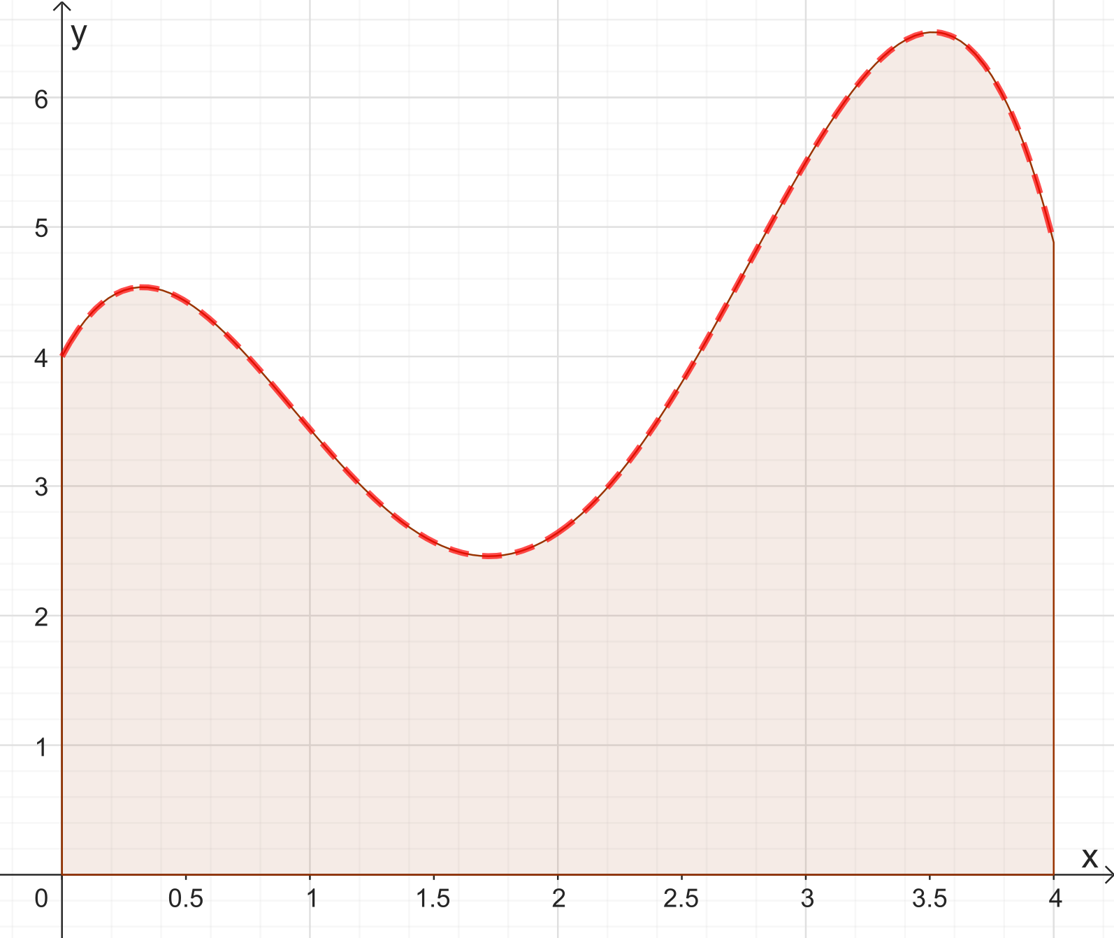
From the graph given in ‎Example 3.1 (part (a)), it is evident that using more subintervals would reduce the instances of areas being either overestimated or underestimated. When you are provided with an illustration of the object for which you are calculating the area, there is virtually no restriction on the number of subintervals you can use when applying Simpson's rule, except for practical limitations such as time or resource constraints. In theory, you can divide the curve into as many subsegments as needed to achieve a highly precise estimation of the area.

However, when applying Simpson's rule to a set of data points measured at a work site, it is important to note that interpolation (estimating values between consecutive observations) is not permitted. Unlike when we have an illustration of the object, where we can visually understand the shape and make informed decisions about subintervals, the lack of a visual representation restricts our ability to accurately interpolate data points in between the observed values, as demonstrated in ‎Example 3.2.

Example 3.2

The owner of a botanical garden would like a price quote for top soil needed on a section of land. Rather than physically visiting the garden, the distributor asks the owner to take nine width measurements, five feet apart, along the total length of the space. Each measurement was taken perpendicular to the length line and was recorded in the order it was taken (the data is summarized below in feet). Using Simpson's rule, approximate the total surface area of this region of land that the distributor will use to quote the client.

24

32

38

41

40

37

34

32

31

Solution

Since there are nine observations taken five feet apart and the first observation starts at 0 ft. along the horizontal length line, the garden must be 40 feet wide. Since a table of values is given, and not an actual scaled photo of the garden, the least \(h\) can be is five; this occurs when \(n=8\). Choosing a larger even \(n\) is not permitted in this case because it will result in subinterval lengths (\(h\)) being shorter than five feet – this data does not exist.

• Can we use even \(n\) values that are less than 8? (Use the comment section below to give your insight!)

Applying Simpson's rule (Equation ‎3.1):

24	32	38	41	40	37	34	32	31
First	Even	Odd	Even	Odd	Even	Odd	Even	Last

\[A_{\mathrm{total}} \approx \frac{h}{3} \times \left[(y_0+y_n)+2(y_2\;+...+\;y_{n-2})+4(y_1\;+...+\;y_{n-1}))\right]\]

\[A_{\mathrm{total}} \approx \frac{5}{3} \times \left[(24+31)+2(38+40+34)+4(32+41+37+31)\right]\]

\[A_{\mathrm{total}} \approx \frac{5}{3} \times 843\]

\[A_{\mathrm{total}} \approx 1405\;\mathrm{ft.}^2\]

Therefore, the garden space covers approximately 1405 sq. feet.

There are several known variants of Simpson's rule, including one that uses third-degree polynomials rather parabolas and another that allows the use of unequal intervals (Easa, 1988). For most trade-related applications, however, the standard version of Simpson's rule presented here, utilizing parabolic segments and equally spaced intervals, offers a practical and reliable method for estimating areas of irregular shapes.

Video Demonstration

The two videos below illustrate how Simpson's rule can be applied to find the area. The video under Question 1 mentions the 'prismoidal formula' in the introduction, although it should not be mistaken with the Simpson's rule. The prismoidal formula is used to calculate the volume of irregularly shaped solids. In retrospect, mentioning the prismoidal formula was a mistake, but that should not detract from the overall message of the video. Furthermore, in both videos we see the formula written in function notation (e.g. we see \(f(x_n)\) rather than \(y_n\)). This does not change how the Simpson's rule is applied; as an exercise, try doing the problems using the notation outlined in this article.

Question 1

Question 2

Question 3 (Advanced)

https://www.youtube.com/watch?v=NShwzjTBOzY

Source

Easa, S. (1988). Area of irregular region with unequal intervals. Journal of Surveying Engineering, 114(2), 50-58.

Schwartz, R. (2011). Thomas Simpson, Weaver and Mathematician. The Right Angle, 18, 6.