Transcript
Table of Contents
Introduction 3
Objective 3
Theoretical Background 4
Experimental/Simulation Procedure 5
Results and Discussion 6
Trial #1: Tuning Parameters: W=30, Kp1=0.27, Tn=0.2 6
Liquid Level: 6
Flowrate: 7
Trial # 2: Tuning parameters: W=40 , KP=0.27, Tn=0.2 8
Liquid Level: 8
Flow rate: 9
Trial # 3: Tuning Parameters W=45, Kp1=2, Tn=0.2 10
Liquid Level 10
Flow rate: 11
Trial #4: Tuning Parameters : W=30, Kp1=1, Tn=0.2 12
Liquid Level: 12
Flow Rate: 13
Trial #5: Tuning Parameters: W=45, Kp=1, Tn=0.5 14
Liquid Level: 14
Flow rate: 15
Trial #6: Tuning Parameters: W=30, Kp=2, Tn=0.5 16
Liquid Level: 16
Flow Rate: 17
Trial #7: Tuning Parameters: W=60, Kp=0.5, Tn=0.5 18
Liquid Level: 18
Flow Rate: 19
Error Analysis 20
Conclusion and Recommendations 20
References 20
Appendices 20
Raw Data 20
Sample Calculations 20
List of Figures:
Figure 1: Output for Liquid level: W=30, Kp=0.27, Tn=0.2 7
Figure 2 Enhanced Close-up version of figure 1 7
Figure 3: Output for Flowrate(Y2): W=30, Kp=0.27, Tn=0.2 8
Figure 4: Enhanced close-up of Figure 3 8
Figure 5: Output for Liquid Level: W=40, Kp=0.27,Tn=0.2 9
Figure 6: Enhanced Close-up of Figure 5 9
Figure 7: Output for Flow rate: W=40, Kp=0.27,Tn=0.2 10
Figure 8: Enhanced Close-up of Figure 7 10
Figure 9: Output for Liquid Level: W=45, Kp1=2, Tn=0.2 11
Figure 10: Enhanced Close-up of Figure 9 11
Figure 11: Output for Flowrate: W=45, Kp1=2, Tn=0.2 12
Figure 12: Enhanced Close-up of Figure 12 12
Figure 13: Output for Liquid Level: W=30, Kp1=1, Tn=0.2 13
Figure 14: Enhanced version of Figure 13 13
Figure 15: Output for Flowrate : W=30, Kp1=1, Tn=0.2 14
Figure 16: Enhanced Close-up of Figure 15 14
Figure 17: Output for Liquid Level: W=45, Kp=1, Tn=0.5 15
Figure 18: Enhanced Close-up of Figure 17 15
Figure 19: Output for Flow rate: W=45, Kp=1, Tn=0.5 16
Figure 20: Enhanced Close-up of Figure 19 16
Figure 21: Output for Liquid Level: W=30, Kp=2, Tn=0.5 17
Figure 22: Enhanced Close-up of Figure 21 17
Figure 23: Output for Flow rate : W=30, Kp=2, Tn=0.5 18
Figure 24: Enhanced Close-up figure 23 18
Figure 25: Output for Liquid Level: W=60, Kp=0.5, Tn=0.5 19
Figure 26; Enhanced Close-up of Figure 25 19
Figure 27: Output for Flowrate: W=60, Kp=0.5, Tn=0.5 20
Figure 28: Enhanced Close-up of Figure 28 20
Introduction
Objective
The objective for this experiment is to work with the equipment and software and familiarize users with industrial control loop components, and optimization of controller settings using different tuning parameters and combinations.
General Information
The experiment performed in this lab session came with the purpose of teaching students the effects of changing set values in a process for P, PI, and PID controllers. It revolved around the selection of proper tuning parameter selection, and was designed to efficiently measure the effects of variation in any of these variables. It is an effective teaching tool considering the measurements and data are performed automatically via the software in use.
This software was Labview. Labview is an acronym standing for Laboratory Virtual Instrument Engineering Workbench. It has been in use for over 20 years now, and is effective in teaching users how to gather data using computers and the potential points of error for such operations. The Labview package is designed to effectively implement computer-controlled data gathering, as well as analysis. For this experiment, a Labview experiment was designed to control the level of water in two tanks, whether separately or in cascade.
Another component of this experiment was the RT578 machine. This piece of equipment is generally used to facilitate the practical learning in the control of four control variables common in engineering. Of interest to this experiment is the control in level of the tank, which was controlled by the flow rate supplied by the equipment. The objectives attached to this machine and software is familiarising users with industrial control loop components, and optimization of controller settings.
The results seen from this experiment are fairly straight-forward. The experiment revolved around the variation of levels in tanks; appropriately adjusting controller variables showed different pathways that the process would attain the new set level when it was changed to a different desired value. An example of this is the variation in Kp value. When Kp is increased, the control variable deviation is increased, and the control variable output oscillates to a greater extent than when Kp is set at a smaller value. Further examples like this will be shown in the Results and Discussion section of this report.
Theoretical Background
For efficient control of a process, industries use automatic controllers. If multiple variables are being controlled and manipulated simultaneously, it will be impossible to avoid interactions amongst them. For this purpose, complex control systems have been implemented have been implemented for a number of industrial models either practically or theoretically. Labview is a software widely used for this particular type of modelling. It will show the variations in process based on changing a number of process variables, and the functioning systems for each of the controllers in use.
Here, the functioning system is an ordinary control system. The system will measure the controlled variable, compare this measurement with the set point, and if there is a difference between the two, changes will be made to the output signal to the manipulated variable in order to eliminate the error. It is a feedback control type of system, attempting to account for variance in control variable by changing the manipulated one. It is very common that feedback control systems (loops) can never achieve perfect control of a process; that is, to keep the output of the process continuously at the desired set point. In a feedback loop system, no corrective action is taken until after a deviation in the controlled variable occurs. This means that perfect control, where the controlled variable does not deviate from the set point during disturbances or set-point changes is theoretically impossible. The control variable will continuously oscillate around the value of the set-point. In this particular experiment, the control variable was the water level in the tank, and the manipulated variable was the work done by the pump supplying water to the tank.
Experimental/Simulation Procedure
Present the procedure of the experiment
Any deviation from lab manual
The experiment procedure included three parts: the start-up, running the experiment via the software, and appropriately shutting down the system. Most of the laboratory work was performed on Labview, changing the parameters for operation control of the process.
Start-Up
The first step in this experiment was checking to make sure the right valves were turned to OPEN/CLOSE in order for the experiment to run. This was done with the help of the TA using the RT578 Instruction Manual.
The computer was then turned ON, and the Labview Software was opened.
In Labview, the file “Level Control” was selected.
In the Labview software, the following initial settings were defined for the experiment:
Kp1
0.27
Tn1
0.2 sec
Tv1
0.0 sec
w1
30%
The pump was then turned on and the water level in the tank was allowed to reach a steady level in the tank (set at 30%).
Experiment Runs on Labview Software
The type of readings for the process was to be “Continuous” – this was selected on the Labview software.
A new Excel file was created on the Desktop – this would be the file where the Labview software would automatically record the results of the experimental runs.
The data for any of the runs could be sent to the Excel file by clicking “New Set in Open File” at the beginning of that particular run.
For this experiment, the values of Kp1, Tn1, and Tv1 were changed while the level in the tank (control variable, w1) was different for each particular run. The results to be measured were the methods of reaching the set point (or close to set point) of each run based off of the values for the PID controller.
It is important that, for each time the set point was changed in order to measure the effects of variation in the PID controller variables with it, the run be properly recorded by selecting “New Set in Open File” on the Labview software.
Shut Down Of System
The shutdown was fairly simple: the first step was to simply turn off the pump.
The Labview program was then closed; the Excel file was checked first to ensure all values from experiment were properly recorded.
The Excel file was copied onto a USB so that the data could be used for calculation of results.
The computer was then turned off, and power to the machine was turned OFF as well.
Results and Discussion
Trial #1: Tuning Parameters: W=30, Kp1=0.27, Tn=0.2
Liquid Level:
Figure 1: Output for Liquid level: W=30, Kp=0.27, Tn=0.2
Figure 2 Enhanced Close-up version of figure 1
Flowrate:
Figure 3: Output for Flowrate(Y2): W=30, Kp=0.27, Tn=0.2
Figure 4: Enhanced close-up of Figure 3
Trial # 2: Tuning parameters: W=40 , KP=0.27, Tn=0.2
Liquid Level:
Figure 5: Output for Liquid Level: W=40, Kp=0.27,Tn=0.2
Figure 6: Enhanced Close-up of Figure 5
Flow rate:
Figure 7: Output for Flow rate: W=40, Kp=0.27,Tn=0.2
Figure 8: Enhanced Close-up of Figure 7
Trial # 3: Tuning Parameters W=45, Kp1=2, Tn=0.2
Liquid Level
Figure 9: Output for Liquid Level: W=45, Kp1=2, Tn=0.2
Figure 10: Enhanced Close-up of Figure 9
Flow rate:
Figure 11: Output for Flowrate: W=45, Kp1=2, Tn=0.2
Figure 12: Enhanced Close-up of Figure 12
Trial #4: Tuning Parameters : W=30, Kp1=1, Tn=0.2
Liquid Level:
Figure 13: Output for Liquid Level: W=30, Kp1=1, Tn=0.2
Figure 14: Enhanced version of Figure 13
Flow Rate:
Figure 15: Output for Flowrate : W=30, Kp1=1, Tn=0.2
Figure 16: Enhanced Close-up of Figure 15
Trial #5: Tuning Parameters: W=45, Kp=1, Tn=0.5
Liquid Level:
Figure 17: Output for Liquid Level: W=45, Kp=1, Tn=0.5
Figure 18: Enhanced Close-up of Figure 17
Flow rate:
Figure 19: Output for Flow rate: W=45, Kp=1, Tn=0.5
Figure 20: Enhanced Close-up of Figure 19
Trial #6: Tuning Parameters: W=30, Kp=2, Tn=0.5
Liquid Level:
Figure 21: Output for Liquid Level: W=30, Kp=2, Tn=0.5
Figure 22: Enhanced Close-up of Figure 21
Flow Rate:
Figure 23: Output for Flow rate : W=30, Kp=2, Tn=0.5
Figure 24: Enhanced Close-up figure 23
Trial #7: Tuning Parameters: W=60, Kp=0.5, Tn=0.5
Liquid Level:
Figure 25: Output for Liquid Level: W=60, Kp=0.5, Tn=0.5
Figure 26; Enhanced Close-up of Figure 25
Flow Rate:
Figure 27: Output for Flowrate: W=60, Kp=0.5, Tn=0.5
Figure 28: Enhanced Close-up of Figure 28
Discussion:
Error Analysis
Conclusion and Recommendations
References
Dhib, R. (2012). CHE 430: Process Control Laboratory Manual, Ryerson University Chemical Engineering Department
Gunt Hamburg, RT578 Instruction Manual, 2013.
Srinivas, P., Lakshmi, K.V. (2012). Modelling and Simulation of Complex Control Systems Using Labview, International Journal of Control Theory and Computer Modelling, 2 (4).