Transcript
4.6 Normal Approximation to the Binomial
For a very large n, we can use the normal distribution to approximate binomial probabilities.
What is large? Approaching infinity
In reality, if np > 5 and n(1-p) > 5, the binomial approximation can be used.
If X be a binomial variable with parameters n and p such that np > 5 and n(1-p) > 5, then X is approximately normally distributed with mean m=np and variance s2=np(1-p). We can then use the standard normal table to get probabilities.
Note: We are going to be modeling a discrete variable using a continuous one, so we need to use a continuity correction factor of .5 when finding our answers.
Binomial Situation Normal Approximation
P(X > 12) P(X > 11.5)
P(X >12) P(X > 12.5)
P(X < 12) P(X < 12.5)
P(X < 12) P(X < 11.5)
P(X =12) P(11.5 < X < 12.5)
Example:A particularly long traffic light on your morning commute is green 40% of the time as you approach it. Assume that each morning represents an independent trial. Let X represent the number of mornings the light is green over a 30 day period.
Is it appropriate to use the normal approximation?
What is the probability that X is less than 20?
What is the probability that X is greater than 22?
What is the probability that X equals 15?
Other Continuous Distributions
Some random variables are always non-negative and for various reasons yield distributions that are skewed to the right. Such variables include the lengths of time between malfunctions for aircraft engines and the length of time between arrivals at a supermarket checkout line.
The Gamma, Exponential, Chi-squared and Weibull are related distributions that can model such situations.
4.3 Gamma Distribution
The Gamma distribution is partially based on the gamma function.
where a >0
Properties of the gamma function:
For a > 1,
Gamma Probability Function
where x ? 0, a > 0, b > 0
The shape of the distribution changes based on a and b. We can break the shape down based on the value of a, the shape parameter.
Alpha > 1 : This is the most frequently encountered situation, particularly, of course, when ? is an integer. The Gamma density function is then an asymetric bell-shaped curve.
Alpha = 1: The Gamma distribution is then just an exponential distribution.
Alpha < 1: The vertical axis is now an asymptote and the Gamma distribution is monotonously decreasing.
These websites visualize how the shape of the distribution changes as the parameters change:
_http://personal.kenyon.edu/hartlaub/MellonProject/Gamma2.html_
_http://www.aiaccess.net/English/Glossaries/GlosMod/e_gm_gamma_distri.htm_
Observe that ? has a larger influence than ? on the shape of the curve: ? merely stretches the curve horizontally and compresses it vertically. Hence, ? is referred to as the scale parameter.
Mean and Variance of Gamma Distribution:
m = a*b
s2= ab2
Example:
Let X be a gamma random variable with alpha = 3 and beta = 4. What is the expression for the density for X? Find the mean and standard deviation.
4.3 Exponential Distribution
Consider a Poisson process with parameter ?. Let X denote the time of the occurrence of the first event. Then X has an exponential distribution with ? = 1/ ?.
Remember: The Poisson distribution is a model of the number of occurrences of some event in an interval of time from 0 to x.
? ? is called the failure rate
? 1/ ? = b is called the average time to failure
Note: This is a special case of the Gamma Distribution with alpha = 1.
Exponential Probability Function
where x ? 0,
Mean and Variance:
µ = ? = 1/?
?2 = ?2 = 1/?2
Shape of the distribution:
Example: Suppose that an electrical component in an airborne radar system has a useful life described by an exponential distribution with a failure rate 10-4 per hour. (a) What is ?? (b) What is the mean time to failure? (c) What is the probability that the component would fail before its expected life?
4.3 Chi-Squared Distribution
Let X be a Gamma random variable with b= 2 and a = g/2 where g is a positive integer. X is said to have a chi-squared distribution with g degrees of freedom.
Probability Function
, x > 0, g is a positive integer
Mean and Variance:
µ = g ?2 = 2g
What are degrees of freedom?
There are n degrees of freedom (or independent pieces of information) in a random sample. When the data (values from sample) are used to compute the mean, there is 1 less degree of freedom in the information.
This distribution is also used heavily in inference about the variance of a population based on a sample.
When we see , it represents that the area to the right of the chi-squared value is .05. This means that P( c2 > x) = .05.
There is a cumulative distribution table for the Chi-squared distribution.
Degrees of Freedom across the rows
Probabilities appear as column headings
Chi-squared values corresponding to the degrees of freedom and the probabilities are in the center of the table.
Example: Find for 10 degrees of freedom.
4.7 Weibull Distribution
This distribution has been used extensively in reliability engineering as a model of time to failure for electrical and mechanical components and systems.
where x > 0, ? > 0, ? > 0
? The random variable X is the time to failure.
? ? is the average time to failure.
? The general shape of the function resembles that of the Gamma Distribution, but becomes more symmetric as the value of ? increases.
? ? is called the shape parameter. Very hard to find if not given.
? For systems with ? ? 1, failures in the system occur almost right away.
? For systems with ? > 1, failures are more likely to occur later.
Mean and Variance
Example: The time to failure of electric substations in hours of a SUN workstation is modeled by a Weibull distribution with ? = ½ and a know shape parameter ? = ?(.001).
What is the mean time to failure?
What is the probability of failure before twice the expected life?
Reliability – Sec. 4.7 continued
Reliability studies are concerned with assessing whether or not a system functions adequately under the conditions for which it was designed. The variable of interest, X, is the time to failure of a system that cannot be repaired once it fails to operate.
Three functions of interest:
The failure density function, f(t) (often Weibull, Gamma or Exponential)
The reliability function, R(t)
The failure or hazard rate of the distribution, r (rho)
The reliability function is the probability that the component will not fail before time t.
R(t) = 1 – P(Component will fail before time t)
= 1 -
= 1 – F(t), where F(t) is the cumulative distribution function evaluated at t.
The hazard rate function gives a picture of the instantaneous rate of failure at time t given the system was operable prior to this time.
r(t) = f(t)/R(t)
Interpretation of the Hazard Rate:
If r is increasing over an interval, then as time goes by a failure is more likely to occur. “Failure due to wear and tear”
If r is decreasing over an interval, then as time goes by, a failure is less likely to occur than it was earlier in the time interval. “Failure due to defects”
A steady hazard rate is expected over the useful life span of a component. “Failure due to random factors”
Often, we have an idea of r and want to derive the failure density and reliability function.
and f(t) = r(t)*R(t)
Example: The length of time in hours that a rechargeable calculator battery will hold its charge is a random variable. Assume that this variable has a Weibull distribution with alpha = .01 and beta = 2.
What is the density function for X?
What is the reliability function for this random variable?
What is the reliability of such a battery at t = 3 hours?
What is the reliability of such a battery at t=12 hours?
What is the reliability of such a battery at t = 20 hours?
What is the hazard rate function for these batteries?
What is the instantaneous rate of failure at t = 3 hours?
What is the instantaneous rate of failure at t = 12
hours?
What is the instantaneous rate of failure at t = 20
hours?
(j) Is the hazard rate function an increasing or decreasing function? Does this seem reasonable from a practical point of view?
Reliability of Series and Parallel System
Series system: A system whose components are arranged in such a way that the system fails when any of its components fail.
Consider a system consisting of k components connected in series. Let Ri(t) denote the reliability of component I. Assume the components are independent in the sense that the reliability of one does not affect the reliability of the others.
The reliability of the entire system is the probability that the system will not fail before time t. The system will not fail IF and ONLY IF no component fails before time t.
Reliability of the system Rs(t) =
Example: It is assumed that the functioning of each component of the system, C1 and C2, is independent. The probability that C1 is working at any given time is 0.90. For C2, this probability is 0.95. What is the probability that the system is functional at any given time?
Parallel System: A system whose components are arranged in such a way that the system fails only if all of its components fail.
The reliability of the entire system is the probability at least one of the components will not fail before time t. The system will fail IF and ONLY IF all components fail before time t.
Reliability of the system Rs(t) = 1 – P(all components fail)
=
Example: It is assumed that the functioning of each component of the system, C1 and C2, is independent. The probability that C1 is working at any given time is 0.90. For C2, this probability is 0.95. What is the probability that the system is functional at any given time?
Complex or Combination System: mixture of series and parallel components
Moment Generating Functions for Continuous Distributions
(in various sections in chapter 4)
Uniform distribution:
Normal distribution:
Gamma distribution:
Chi-squared distribution:
Note this is a Gamma with a=g/2 and b = 2
Exponential distribution:
Note this is a Gamma with a=1
Comparing Data to Continuous Distributions (not in book)
We can plot the probability distribution versus the data we observe to see how they compare or we can use moment generating functions.
EXAMPLE 1
The following data are the percent manganese in 125 different casts from a blast furnace.
1.40 1.44 1.42 1.72 1.34 1.50 1.50 1.48 1.16 1.28 1.32 1.22 1.28 1.46 1.58 1.60 1.38 1.46 1.46 1.36 1.54 1.30 1.22 1.24 1.36 1.50 1.70 1.62 1.34 1.28 1.34 1.38 1.24 1.52 1.72 1.22 1.38 1.38 1.62 1.46 1.36 1.18 1.40 1.32 1.22 1.76 1.18 1.34 1.44 1.54 1.58 1.38 1.58 1.28 1.50 1.40 1.20 1.16 1.36 1.40 1.50 1.62 1.42 1.38 1.26 1.42 1.40 1.30 1.28 1.44 1.34 1.48 1.76 1.38 1.34 1.50 1.38 1.26 1.36 1.48 1.28 1.54 1.52 1.68 1.60 1.28 1.52 1.36 1.26 1.30 1.46 1.10 1.44 1.58 1.68 1.44 1.08 1.38 1.38 1.16 1.48 1.48 1.06 1.46 1.52 1.66 1.46 1.08 1.50 1.42 1.34 1.28 1.42 1.10 1.80 1.46 1.62 1.38 1.36 1.52 1.34 1.40 1.18 1.36 1.16
Does the normal distribution seem to match the data?
EXAMPLE 2
The following data are bearing load lives (in millions of revolutions) listed in increasing order for M50 bearings with silicon nitride ceramic balls tested at a 6.45 kN load.
47.1 67.3 69.1 90.8 103.6 106.0 115.0 126.0
146.6 229.0 239.6 240.0 275.1 278.0 289.0 293.9
367.0 385.9 392.0 505.0
Does the Normal or Weibull distribution seem more appropriate?
EXAMPLE 3
The following data are the times between successive failures of the air-conditioning systems in a fleet of 13 Boeing 720 jet aircraft. In the table “a” indicates a major overhaul.
Plane identification number
7907 7908 7909 7910 7911 7912 7913 7914 7915 7916 7917 8044 8045
194 413 90 74 55 23 97 50 359 50 130 487 102
15 14 10 57 320 261 51 44 9 254 493 18 209
41 58 60 48 56 87 11 102 12 5
100 14
29 37 186 29 104 7 4 72 270 283
7 57
33 100 61 502 220 120 141 22 603 35
98 54
181 65 49 12 239 14 18 39 3 12
5 32
9 14 70 47 62 142 3 104
85 67
169 24 21 246 47 68 15 2
91 59
447 56 29 176 225 77 197 438
43 134
184 20 386 182 71 80 188
230 152
36 49 59 33 246 1 79
3 27
201 84 27 a 21 16 88
130 14
118 44 a 15 42 106 46
230
a 59 153 104 20 206 5
66
34 29 26 35 5 82 5
61
31 118 326
12 54 36
34
18 25
120 31 22
67 156
11 216 139
57 310
3 46 210
62 76
14 111 97
7 26
71 39 30
22 44
11 63 23
34 23
14 18 13
62
11 191 14
a
16 18
130
90 163
208
1 24
70
16
101
52
208
95
Exponential Distribution