Chapter 6: The Production, Cost, and Technology of Health Care

Chapter 6: The Production, Cost, and Technology of Health Care This chapter relies on several key concepts from Chapter 2 including production functions, isoquants, isocost curves, marginal cost, average cost, and elasticity. An outline for the relevant sections of chapter 2 is included at the end of this outline (since elasticity was referred to previously in other chapters, it will not be included again). Production and the Possibilities for Substitution Substitution Does it mean the inputs are the same? 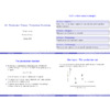This does not mean that the two inputs are equivalent, but only that alternative combinations are possible Review Figure 6-1. (Note: Isoquants are introduced in chapter 2). How do panel A and panel B reveal different production capabilities for whether the inputs can be substituted? In panel A, 0 physician hours are required to produce one case and the addition of nursing hours will not add to output unless physician hours are also increased. This applies to a production problem since patient care requires certain tasks only a physician can perform and additional nurses added would be a wasted resource. In panel B, many combinations of inputs could be chosen without being wasteful. In Panel A: note that P and N refer to the number of physician hours (P) and nurse hours (N) required to treat one patient (since Q=1). Do additional hours (or fewer hours) of only one input increase the number of patients that can be treated? No. If P increased (rising above M), only one patient is still treated because N has not changed. The producer does not move to a different isoquant, but moves ALONG the current isoquant. If N increased (moving to the right of M), only one patient is still treated because P has not changed. The producer does not move to a different isoquant, but moves ALONG the current isoquant. Using more of one input does NOT yield more output. ALSO, specific minimum amounts of P and N must be used to produce Q=1 output. Although (unnecessary) inputs can be added, at least P and N amounts must be used. In Panel B: can P and N be substituted for each other to treat the patient? Note there are many different combinations of P and N that could be used to treat one patient. Moving from the combination of inputs (N, P) that correspond to Point Y on the isoquant, if P increasing, holding N constant, the producer would move “above” the current isoquant. But, the producer can also MOVE ALONG the isoquant and substitute P for N (or N for P depending on the direction). Starting at point Y, the producer can use a different combination identified as point Z that uses (S, R) amounts of input for nurse hours and physician hours to maintain production of 1 unit of output. Substitution is possible. The slope of the isoquant (MRTS from chapter 2), indicates how much substitution is possible. What Degree of Substitution is Possible? Review Box 6-1: “Health Care Professional: Expanding the Possibilities” What does division of labor refer to? Variety of specializations among allied health labor. Adam Smith’s theory explains how a focus by each expert on his/her specialized task yields greater output for the whole than were one to insist that each person be a generalist. Is substitution possible? Yes, availability of other health professionals enhances possibilities for substitution in production (i.e. nurse practitioners and PA’s can substitute for physician time). Are there limits to the substitutability of resources? Yes, there are some limits but substitution could be substantial Elasticity of Substitution What does it measure? (What is the definition?) Elasticity of substitution measures the responsiveness of a cost minimizing firm to changes in relative input prices How is it measured/calculated? Es=%change in factor input ratio% change in factor price ratio The discussion in the text applies values to Figure 6.1 on p. 135. You might want to draw this figure then add the values referenced to the figure while you are reading the examples. Initially: Hospital employs 100 physicians, P=100. Hospital employs 100 nurses, N=100. The factor input ratio is P/N=100/100=1.0. Physician wages (Pp) = 200,000. Nurse wage (Pn) = 40,000 The factor price ratio = 200,00/40,000 = 5.0 If physician wages increase 10% then: Hospital employs 99 physicians, P=9. Hospital employs 105 nurses, N=105. The factor input ratio is P/N=99/105=0.94. The percentage change in the factor input ratio is (0.94-1.00)/1.0 = -0.06 (or 6%) Physician wages (Pp) = 220,000. Nurse wage (Pn) = 40,000 The factor price ratio = 220,000/40,000 = 5.5 The percentage change in the factor price ratio is (5.5-5.0)/5.0 = 0.10 (or 10%) So the Elasticity of Substitution is Es = -0.06/0.10 = -0.60. Note: the elasticity is negative because of the direction of the change but the elasticity is reported in absolute value to interpret the size, |-0.60| = 0.60 See the discussion about if Es=0.6 then a 1% increase in the relative prices yields a 0.6% change in the relative mix of factor inputs. So, if the input ratio changes, then the elasticity of substitution indicates how the ratio of factor inputs changes. In this example, the hospital chooses to replace 1 physician, whose wage would have been $220,000, with 5 nurses, whose wages are only $40,000 each (for a total of $200,000), which would save the hospital $20,000 (P.137) What does an elasticity of 0 indicate? Perfectly inelastic; an elasticity of substitution equal to zero will use the same input combination to produce a given level of output regardless of relative factor prices; higher values of ES indicate a greater potential for substitutability. What did Acemoglu and Finkelstein (2006) find about how health care firms responded to changes in labor cost? They found that healthcare firms responded to the introduction of the Medicare payment system by increasing the capital/labor ratio. Estimates for Hospital Care Review Table 6-1. Do the values indicate substitutability between the inputs? The elasticities reported are at least sufficient to show that some suitability exists between virtually all pairs of hospital inputs. Costs in Theory and Practice Deriving the Cost Function: NOTE: you do not need to be able to draw the isocost curves and isoquants yourself, but need to be able to read the graphs when provided. Review Figure 6-2. How many isoquants are in figure 6-2 (a)? 3 Which isoquant corresponds to the highest output level? Q=200 Which point of tangency corresponds to highest output level that can be produced and which isocost is relevant for producing that output? Point G; isocost HI Can you identify the minimum cost of producing the various levels of Q on the isoquants? (Locate the point of tangency between the isoquant and the isocost curve). Cost Minimization Review Figure 6-2. How many isocosts are in figure 6-2 (a)? 3 What letters identify the endpoints of the isocosts? AB, DE, and HI Which isocost indicates the highest cost? HI Then, given the prices w and r, how is the total cost calculated for using different levels of L and K? What is the general equation? TC= rK + wL (r=rental price of capital & w=wage rate of labor) Use the example in the middle of p. 140 to complete the cost equation for the specific example of producing 100 visits. TC=1200*25+1000*20 What is the total cost? TC=$50,000 What is the cost minimizing input combination to produce 150 visits? At point F k=40 and L=30 What is the cost of producing those 150 visits? TC=1200*40+1000*30=$78,000 Economies of Scale and Scope Review Figure 6-3. How is long-run average cost (LRAC) calculated from the total cost? Dividing total cost by # of physician visits What are economies of scale? When its LRAC is declining as output increases What are diseconomies of scale? If and only if LRAC is increasing as output is increasing Can you identify where in Figure 6-3 economies of scale occur? AB What are economies of scope? possible only for multi-producing firm; occurs whenever it’s possible to produce jointly two or more goods more cheaply than if we produce them separately Why are economies of scope relevant in health care? b/c many healthcare firms are multi-producing in nature Review equation 6.1. Why would Economies of Scale and Scope be Important? Why do economists promote the theory of competition? competition forces the firm in the long run to operate so that it minimizes average costs Do most health care firms operate in perfectly competitive markets? No Review Figure 6.3. What is a “natural monopoly”? (Review the example in the text.) Empirical Cost-Function Studies Long-run versus Short-run Studies: How does the long-run differ from the short-run? long-run = permits a firm to vary all factors of production; short-run = situations in which a firm isn’t able to vary all inputs and at least one factor of production is fixed Structural versus Behavioral Cost Functions: do the studies indicates whether economies of scale exist? Difficulties Faced by All Hospital Cost Studies What are some of the difficulties? Hospitals differ by types of cases they treat (case-mix problems) how to treat quality lack of reliable measures of hospital input prices almost always omit physicians input prices completely Review figure 6.4. Modern Results: what are the current conclusions? economies of scale exist in hospitals; found significant savings for mergers 2-4 years after consolidation Summary: Empirical Cost Studies and Economies of Scale Technical and Allocative Inefficiency Technical Inefficiency Review Figure 6-5. What does technical inefficiency refer to? occurs when the firm produces the max possible sustained output from a given set of inputs (technically inefficient firms fall of their frontier) How is it observed in a graph when one input is used in production? seen in panel A, firms on the production frontier f(L) are considered technically eff. (firms 4 & 5), firms off the frontier are technically ineff. (firms 1-3) How is it observed in a graph when two inputs are used in production? seen in panel B, shows an isoquant treating a certain # of cases, firms 6 & 7 are on the isoquant and thus represent technical ineff., firms 8-10 are off the isoquant, have employed more input quantities than technically efficient production requires Allocative Inefficiency Review Figure 6-6. What does allocative inefficiency refer to? situations in which either inputs or outputs are put to their best possible uses in the economy so that no further gains in output or welfare are possible How do you identify allocative efficiency graphically? Why is Point A technically efficient but allocatively inefficient? (What are you looking for in the graph?) at current input prices it uses too much capital and not enough labor Why is Point B both technically and allocatively efficient? reduces cost but produces same 100 cases; equality of ratio of input prices to ratio of marginal products Frontier Analysis (SKIP THIS SECTION) The Uses of Hospital Efficiency Studies Total Hospital Efficiency: how efficient are hospitals? For-Profit versus Nonprofit Hospitals: is there a relationship between status and efficiency? Efficiency and Hospital Quality What measure of “quality” is used by Deily and McKay (2006)? What did Deily and McKay find about the relationship between inefficiency and quality? Are Hospital Frontier Efficiency Studies Reliable? (SKIP THIS SECTION) Performance-Based Budgeting: how might efficiency be used to create incentives for hospitals? Box 6-2: “Should We Close Inefficient Hospitals?”—what does the research indicate about the overall effect? Technological Changes and Costs Technological Change: Cost Increasing or Decreasing? Review Figure 6-9. In Panel A, how can you identify graphically that the technological change was cost-decreasing? inward isoquant shift (isocost from $68,000 to $42,000) In Panel B, how can you identify graphically that the technological change was cost-increasing? outward isoquant shift (isocost from $50,000 to $71,000) Health Care Price Increases When Technological Change Occurs Is all “technological change” cost increasing? Read Box 6-3: Aspirin, the Wonder Drug at a Bargain What is the difficulty in measuring the change in cost of technological change over time? Can the cost of treatment in one time period simply be compared to the cost in a different time? How is a price index affected by what is included in its calculation? Does the research suggest quality and technological improvements are appropriately accounted for when using a price index? Review Table 6-2. What role should quality of life play in comparing the relative costs of a treatment over time? Diffusion of New Health Care Technologies Who Adopts and Why What is the “profit principle”? physicians tend to adopt a new surgicial technique if they expect to increase their revenue What is the “information channel” explanation? emphasizes role of friends, colleagues, journals & conferences in informing and encouraging the adoption decision What are “information externalities”? uncompensated, beneficial effect on a third person caused by actions of a market How quickly does new technology get adopted and who is the most likely to adopt it? occurs slow at first, then at increasing rate that continues at a decreasing rate approaching its limits and the adopters tend to be younger people Other Factors That May Affect Adoption Rates: what are they? Diffusion of Technology and Managed Care: how has managed care affected the adoption of technology? Conclusions Suggested End-of-Chapter Questions Discussion Questions: 3 and 9 How do legal restrictions on practice for nurses and physicians tend to affect the observed elasticities of substitution? Would the elasticities be higher if legal restrictions were removed? Would quality of care be affected? Legal restriction on the practice of nurses and physicians limits the supply and increases the factor price. This reduces the elasticity of substitution because already a small number of physicians and nurses would be serving in the market and further reduction would be difficult. The opposite would happen if legal restrictions are removed. If legal restrictions are removed, the factor price would be cheaper and more physicians would be employed by hospitals. They would replace other expensive factor inputs and quality of care would be improved because physicians and nurses would bring better skills to the table. Which of the following types of technological change in health care are likely to be cost increasing: threats of malpractice suits that cause physicians to order more diagnostic tests on average for a given set of patient symptoms The technological change would be cost increasing because marginal benefit from ordering more tests than required would be very small as compared to marginal costs a new computer-assisted scanning device that enables physicians to take much more detailed pictures of the brain This technological change could be cost decreasing because the scanning is computer assisted and would not require much labor input. So, the cost is low. As far as benefit is concerned, it might be helpful in diagnosing diseases, which previously required more tests and can save more patient life. Hence, benefit outweighs cost in this case which reduces overall costs. the introduction of penicillin earlier in this century This technological change could be cost decreasing because penicillin is a cheap medicine, which would have avoided a lot of deaths. Hence, benefit outweighs the cost. greater emphasis on preventive care? Discuss. Greater emphasis on preventative care would decrease cost as a lot of curative care would not be required. Preventative care is generally cheap as it requires a healthy lifestyle, knowledge of diseases which can be easily transferred technologically. Very high savings can be achieved if curative care is not required. Exercises: 3, 4, 5, and 8 (use the prices referred to on p. 111 to calculate the total cost, and then the average cost of production for the input levels) Determine the elasticity of substitution in the case of the isoquant in panel A of Figure 6.1. If the isoquant is L-shaped isoquant, it means that capital and labor needs to be used in a fixed proportion, no matter what. It implies that price change would not have an effect on the combination of two inputs required to produce a given output. The elasticity of substitution is given as: E=percentage change in factor input ratiopercentage change in factor price ratio If price change would not have any effect on factor input ratio, then change in factor input ratio would be zero. Hence, elasticity of substitution would be zero. Suppose a firm has the production technology shown below for Goods 1 and 2. Does Good 1 indicate economies of scale? Why? Good 1 does not depict a case of economies of scale but a case of constant returns to scale because the rate of increase of output is the same as the rate of increase of input. Does Good 2 indicate economies of scale? Why? Good 2 does depict a case of economies of because the rate of increase of output is more than the rate of increase of output. Do the two goods indicate economies of scope? Why? Both the goods together make a case for economies of scope. Because the cost of producing both goods together is less than producing the same amount of goods separately. In this table, cost of producing 10 units of each good separately costs 110 but together costs 100 only. Same logic applies for two other cases. If any firm’s price of labor and capital each double, what will happen to the expansion path (i.e., locus of tangencies between the isoquants and isocost curves)? What will happen to the firm’s average cost curve? The expansion path represents the total cost curve for product with total costs on y-axis and with quantity on x-axis. If the costs of both inputs double, then half the output would be produced at the same cost. Hence, the expansion path would contract by 50% along the x-axis. Average cost is the ratio of sum of fixed cost and variable cost with the total quantity produced. Hence, the starting point of average cost would be the same i. e. fixed cost. After that the average cost curve would move upwards as compared to previous curve. The change is illustrated in Figure one below. Calculate the average costs at points C, F, and G in Figure 6.2. Do they imply increasing or decreasing returns to scale? Why? The total cost is given by the function of capital and labor as below. In this case value of price of factor inputs is given. TC = rK + wL TC = 1200K + 1000L (now calculate the total cost for each point as below) TCC = 1200 * 25 + 1000 * 20 = $50,000 TCF = 1200 * 40 + 1000 * 30 = $78,000 TCG = 1200 * 50 + 1000 * 45 = $105,000 (now calculate the average cost for each point as below) ACC = $50,000100=$500 ACF = $78,000150=$520 ACG = $105,000200=$525 It is evident that the average cost is rising with increase in quantity and hence this a case of decreasing returns to scale. Note: Exercise 3 hint, is there any substitutability? Exercise 4: parts a and b, the total cost is provided for each quantity so you just have to convert to the average and apply the definition to each of the goods to see if economies of scale exist. For part c, you have to apply the concept described on p. 141 that is shown in equation 6.1. You have the costs of producing quantities of goods 1 and 2 separately, and then the cost if they are produced jointly, so are costs higher or lower when produced jointly? Exercise 5: if prices of both double, does the slope change? Would the answer differ if only one price changed? Exercise 8: this exercise requires you to apply the quantities shown in the figure with the input prices described in the text to calculate the total cost, then find the average cost. You then have to apply the concept of economies of scale to determine if there are increasing or decreasing returns to scale. Chapter 2: Microeconomic Tools for Health Economics Note: this chapter is a brief summary/review of many of the topics covered in a principles of microeconomics course. You should refer to an introductory level textbook (or in some cases an intermediate level) if you need more information about these topics. Production and Market Supply (p. 46) The Production Function What is a production function? Review Figure 2-13. What is marginal product (MP)? How is MP represented graphically? Is MP constant, increasing, or decreasing in the figure? What is the law of diminishing returns? Production Functions Review Table 2-4. In this production schedule, notice one of the inputs is used in fixed quantity so only one input is variable (this identifies production is in the “short-run” since all inputs can be varied in the long-run) How is MP calculated? How is AP calculated? Using equation 2.12 (in the middle of the page), can you confirm the calculation of Q using the K and L values in the table? Review Table 2-5 and Figure 2-14. What is an isoquant? (NOTE: graphically these curves looks similar to indifference curves but they represent PRODUCTION, not consumption) Notice this isoquant schedule identifies the different combinations of inputs that yield the same quantity of output (quantity of 10 here). Since both K and L are variable, isoquants indicate long-run production capabilities (POSSIBLE production until a level of one of the inputs is selected and a short-run production phase is entered). What does the marginal rate of technical substitution (MRTS) measure? Is substitution possible in practice? Isocost Curves What is an isocost curve? Is an isocost curve similar to a budget constraint? Review equation 2.13, the example underneath, then equation 2.14 and 2.15. How do you determine the vertical endpoint of the isocost curve? How do you determine the horizontal endpoint of the isocost curve? Cost Minimization or Output Maximization The producer’s goal can be viewed as either cost minimizing or output maximizing. Cost minimizing means producing a given amount of Q for minimum cost. Output maximizing means producing the maximum quantity possible for a given amount of total cost. Review Figure 2-15. How can you use the graph of the isocost curve and the isoquant to determine the optimal amounts of K and L to use to produce Q? Marginal and Average Cost Curves Note: these curves indicate they are LONG-RUN cost curves, not short-run cost curves. How does the short run differ from the long run? What does “economies of scale” refer to? What would the long-run average cost (LRAC) curve look like if economies of scale exist? Why might economies of scale occur? In Figure 2.16, does the producer have economies of scale for all quantities of output? (HINT: No.) Where in this figure are economies of scale experienced?