Transcript
288Miller•Economics Today, Nineteenth Edition
Chapter 19Demand and Supply Elasticity287
Answers to Questions for Critical Analysis
The Price Elasticity of Demand for Cable TV Subscriptions (p. 418)
Why does it make sense that there was a negative percentage change in the quantity of cable TV subscriptions demanded in response to an increase in the price of these subscriptions?
According to the law of demand, the quantity demanded reduces in response to an increase in price. For this reason, an increase in the price of cable TV subscriptions results in a negative percentage change in the quantity of cable TV subscriptions.
The Price Elasticity of Demand for Movie Tickets (p. 419)
Would the estimated price elasticity of demand for movie tickets have been different if we had not used the average-values formula? How?
Percent Change in Quantity Demanded = Change in Quantity Demanded/Original Quantity Demanded
= (1.34 billion - 1.26 billion)/1.34 billion = 0.0597
Percent Change in Price = Change in Price/Original Price
= ($8.08 - $7.84)/$7.84 = 0.0306
EP = Percent Change in Quantity Demanded/Percent Change in Price
= 0.0597/0.0306 = 1.95
If we had not used the average-values formula, the estimated price elasticity of demand for peanuts would have been lower at 1.95 instead of 2.04.
Short-Term Stress and the Price Elasticity of Demand for Alcohol (p. 426)
How do you think that reducing experimental subjects’ stress would have affected their price elasticity of demand for alcohol?
Reducing experimental subjects’ stress makes them less sensitive to an increase in the price of alcohol. This means a lower price elasticity of demand for alcohol.
You Are There
Using Price Elasticity of Supply to Assess Effects of Rewards for Academic Performance (pp. 430–431)
1. Why does it make sense that Fryer found a positive percentage change in the amount of learning tasks supplied in response to a rise in the monetary reward for performing them?
A rise in the monetary reward for performing learning tasks provides the students an incentive to increase the number of those tasks they can perform.
2. Is the students’ supply of learning tasks relatively elastic or inelastic? Explain.
A 10 percent increase in incentive payments induces students to perform 8.7 percent more educational tasks. The elasticity of supply of learning tasks is therefore 0.87, meaning that the students’ supply of learning tasks is relatively inelastic.
Issues and Applications
Cotton Subsidies and the Price Elasticity of Cotton Supply in Egypt (p. 431–432)
1. What do you suppose were the likely short-run adjustments to removal of the cotton subsidy by Egyptian farmers who continued to devote all of their lands to agricultural crops?
In the short run, Egyptian farmers who continued to devote all of their lands to agricultural crops would reduce their quantity of cotton supplied.
2. How will the long-run adjustment of Egyptian cotton supply from elimination of the subsidy likely affect the number of suppliers—that is, Egyptian cotton farmers? Explain.
In the long run, the number of Egyptian cotton farmers will decrease, so that the price elasticity of supply would be greater than 2.47—the short-run estimate.
Research Project
1. Learn more about developments in the market for Egyptian cotton in the Web Links in MyEconLab.
2. To obtain data about the markets for various agricultural crops, including cotton crops, see the Web Links in MyEconLab.
Answers to Problems
19-1. When the price of shirts emblazoned with a college logo is $20, consumers buy 150 per week. When the price declines to $19, consumers purchase 200 per week. Based on this information, calculate the price elasticity of demand for logo-emblazoned shirts.
-[(200 ? 150)/(350/2)]/[(19 ? 20)/(39/2)], which is approximately equal to -5.6. Thus, the absolute price elasticity of demand equals 5.6.
19-2. Table 19-2 indicates that the short-run price elasticity of demand for tires is 0.9. If an increase in the price of petroleum (used in producing tires) causes the market prices of tires to rise from $50 to $60, by what percentage would you expect the quantity of tires demanded to change?
To calculate the increase in tire prices using our formula for the price elasticity of demand, we take the difference between $60.00 and $50.00, or $10.00, and divide it by the average of the two prices, or $55.00, which yields an 18.2 percent increase. Let X denote the predicted decrease in the quantity. Then X/20 percent = ?0.9. Hence, X = ?16.4 percent.
19-3. The diagram below depicts the demand curve for “miniburgers” in a nationwide fast-food market. Use the information in this diagram to answer the questions that follow.
a. What is the price elasticity of demand along the range of the demand curve between a price of $0.20 per miniburger and a price of $0.40 per miniburger? Is demand elastic or inelastic over this range?
b. What is the price elasticity of demand along the range of the demand curve between a price of $0.80 per miniburger and a price of $1.20 per miniburger? Is demand elastic or inelastic over this range?
c. What is the price elasticity of demand along the range of the demand curve between a price of $1.60 per miniburger and a price of $1.80 per miniburger? Is demand elastic or inelastic over this range?
a. ?[(90 ? 80)/(85)]/[(0.20 ? 0.40)/(0.30)], which is approximately equal to ?0.18. Consequently, the absolute price elasticity of demand is 0.18, so demand is inelastic over this range.
b. ?[(60 ? 40)/(50)]/[(0.80 ? 1.20)/(1.00)] = ?1.00. The absolute price elasticity of demand, therefore, equals 1.00, which implies that demand is unit-elastic over this range.
c. ?[(20 ? 10)/(15)]/[(1.60 ? 1.80)/(1.70)], which is approximately equal to ?5.67. Thus, the absolute price elasticity of demand is 5.67, so demand is elastic over this range.
19-4. In a local market, the monthly price of Internet access service decreases from $20 per account to $10 per account, and the total quantity of monthly accounts across all Internet access providers increases from 100,000 to 200,000. What is the price elasticity of demand? Is demand elastic, unit-elastic, or inelastic?
-[(200,000 - 100,000)/(300,000/2)]/[($10 - $20)/($30/2)] = -1.00. The absolute price elasticity
of demand, therefore, equals 1.00, which implies that demand is unit-elastic over this range.
19-5. At a price of $57.50 to play 18 holes on local golf courses, 1,200 consumers pay to play a game of golf each day. A rise in the price to $62.50 causes the number of consumers to decline to 800. What is the price elasticity of demand? Is demand elastic, unit-elastic, or inelastic?
-[(800 ? 1200)/(2000/2)]/[($62.50 ? $57.50)/($120.00/2)] = -4.8. Hence, the absolute price elasticity of demand equals 4.8. Demand is elastic over this range.
19-6. It is very difficult to find goods with perfectly elastic or perfectly inelastic demand. We can, however, find goods that lie near these extremes. Characterize demands for the following goods as being near perfectly elastic or near perfectly inelastic.
a. Corn grown and harvested by a small farmer in Iowa
b. Heroin for a drug addict
c. Water for a desert hiker
d. One of several optional textbooks in a pass-fail course
a. Nearly perfectly elastic
b. Nearly perfectly inelastic
c. Nearly perfectly inelastic
d. Nearly perfectly elastic
19-7. In the market for hand-made guitars, when the price of guitars is $800, annual revenues are $640,000. When the price falls to $700, annual revenues decline to $630,000. Over this range of guitar prices, is the demand for hand-made guitars elastic, unit-elastic, or inelastic?
Because price and total revenue move in the same direction, then over this range of demand, the demand for hand-made guitars is inelastic.
19-8. Suppose that over a range of prices, the price elasticity of demand varies from 15.0 to 2.5. Over another range of prices, the price elasticity of demand varies from 1.5 to 0.75. What can you say about total revenues and the total revenue curve over these two ranges of the demand curve as price falls?
Within the first range, demand is elastic. As price falls, therefore, total revenues increase. Within the second range, demand is at first elastic and then inelastic. When price falls, therefore, total revenues are initially rising. Eventually, total revenues reach the maximum point, which corresponds to the point of unit elasticity. Beyond this point, total revenues decline.
19-9. Based solely on the information provided below, characterize the demands for the following goods as being more elastic or more inelastic.
a. A 45-cent box of salt that you buy once a year
b. A type of high-powered ski boat that you can rent from any one of a number of rental agencies
c. A specific brand of bottled water
d. Automobile insurance in a state that requires autos to be insured but has only a few insurance companies
e. A 75-cent guitar pick for the lead guitarist of a major rock band
a. More inelastic because it represents a smaller portion of the budget
b. More elastic because there are many close substitutes
c. More elastic, because there are a number of substitutes
d. More inelastic because there are few close substitutes
e. More inelastic because it represents a small portion of the budget
19-10. The value of cross price elasticity of demand between goods X and Y is 1.25, while the cross price elasticity of demand between goods X and Z is –2.0. Characterize X and Y and X and Z as substitutes or complements.
Goods X and Y are substitutes, and goods X and Z are complements.
19-11. Suppose that the cross price elasticity of demand between eggs and bacon is –0.5. What would you expect to happen to purchases of bacon if the price of eggs rises by 10 percent?
Let X denote the percentage change in the quantity of bacon. Then X/10 percent = ?0.5. X, therefore, is ?5 percent. Thus, purchases of bacon would be expected to decrease by 5 percent
19-12. A 5 percent increase in the price of digital apps reduces the amount of tablet devices demanded by 3 percent. What is the cross price elasticity of demand? Are tablet devices and digital apps complements or substitutes?
The cross price elasticity of demand is –3 percent/5 percent = –0.6, so tablet devices and digital apps are complements.
19-13. An individual’s income rises from $80,000 per year to $84,000 per year, and as a consequence, the person’s purchases of movie downloads rise from 48 per year to 72 per year. What is this individual’s income elasticity of demand? Are movie downloads a normal or inferior good? (Hint: You may want to refer to the discussion of normal and inferior goods on page 58 in Chapter 3.)
The income elasticity of demand is equal to [(72 ? 48)/(120/2)]/[($84,000 ? $80,000)/ ($164,000/2)] = +8.2, so downloadable movies are a normal good.
19-14. Assume that the income elasticity of demand for hot dogs is –1.25 and that the income elasticity of demand for lobster is 1.25. Based on the fact that the measure for hot dogs is negative while that for lobster is positive, are these normal or inferior goods?
Income elasticity of demand is measured as the percentage change in demand divided by the percentage change in income. A negative income elasticity of demand indicates that as income rises, demand falls. This type of good is defined in Chapter 3 as an inferior good. A positive income elasticity of demand, therefore, indicates that the good is a normal good, as defined in Chapter 3. Hence, we can conclude that a hot dog is an inferior good and that lobster is a normal good.
19-15. At a price of $25,000, producers of midsized automobiles are willing to manufacture and sell 75,000 cars per month. At a price of $35,000, they are willing to produce and sell 125,000 a month. Using the same type of calculation method used to compute the price elasticity of demand, what is the price elasticity of supply? Is supply elastic, unit-elastic,
or inelastic?
[(125,000 ? 75,000)/(200,000/2)]/[($35,000 ? $25,000)/($60,000/2)] = 1.5. Supply is elastic.
19-16. An increase in the market price of men’s haircuts, from $15 per haircut to $25 per haircut, initially causes a local barbershop to have its employees work overtime to increase the number of daily haircuts provided from 35 to 45. When the $25 market price remains unchanged for several weeks and all other things remain equal as well, the barbershop hires additional employees and provides 65 haircuts per day. What is the short-run price elasticity of supply? What is the long-run price elasticity of supply?
The short-run price elasticity of supply is [(45 - 35)/40] / [($25 - $15)/$20] (1/4) / (1/2) = 2/4
= 0.50, and the long-run price elasticity of supply is [(65 - 35)/50] / [($25 - $15)/$20] = (3/5) / (1/2) = 6/5 = 1.2.
19-17. Consider panel (a) of Figure 19-1. Use the basic definition of the price elasticity of demand to explain why the value of the price elasticity of demand is zero for the extremely rare situation of vertical demand curve?
For any price change along this demand curve, the change in quantity demanded is zero, so the percentage change in quantity demanded is zero. We know that by definition the price elasticity of demand is the percentage change in quantity, which in this case is zero, divided by the percentage change in price, and this ratio equals zero.
19-18. Take a look at Figure 19-2. Work out the calculation for the price elasticity of demand between prices of $11 per reservation and $10 per reservation to prove that the value is 21?
The percentage change in quantity demanded equals (100,000 reservations – 0 reservations) / [(100,000 reservations + 0 reservations)/2] = 10/5 = 2. The percentage change in price equals ($11 per reservation ? $10 per reservation) / [($11 per reservation + $10 per reservation)/2] = 0.01 / 0.105 = 0.0952. Hence, the price elasticity of demand is equal to 2 / 0.0952 = 21.
19-19. Consider Figure 19-2. Work out the calculation for the price elasticity of demand between prices of $1 per reservation and $2 per reservation to prove that the value is 0.158?
The percentage change in quantity demanded equals (1 million reservations – 900,000 reservations) / [(1 million reservations + 900,000 reservations)/2] = 10/95 = 0.1053. The percentage change in price equals ($2 per reservation ? $1 per reservation) / [($2 per reservation + $1 per reservation)/2] = 0.01 / 0.015 = 0.6667. Hence, the price elasticity of demand is equal
to 0.1053/ 0.6667 = 0.158.
19-20. Take a look at Figure 19-2. Work out the calculation for the price elasticity of demand between prices of $6 per reservation and $5 per reservation to prove that the value is 1?
The percentage change in quantity demanded equals (600,000 reservations – 500,000 reservations) / [(600,000 reservations + 500,000 reservations)/2] = 10/55 = 0.182. The percentage change in price equals ($6 per reservation ?$5 per reservation) / [($6 per reservation + $5 per reservation)/2] = 0.01 / 0.055 = 0.182. Hence, the price elasticity of demand is equal to 0.182 / 0.182 = 1.
19-21. Consider Figure 19-3. Following a price increase, is the quantity demanded more responsive to the price increase immediately, after an initial passage of time, and then after even more time has passed? Why is this so?
The quantity demanded is least responsive to the immediate price change, more responsive after an initial passage of time, and even more responsive after even more time has passed. This is so because as more and more time is available for adjustment to the price increase, buyers can more readily find substitutes for this particular good or service.
19-22. Take a look at Figure 19-5. Following a price increase, is the quantity supplied more responsive to the price increase immediately, after an initial passage of time, and then after even more time has passed? Why is this so?
The quantity supplied is least responsive to the immediate price change, more responsive after an initial passage of time, and even more responsive after even more time has passed. As more time initially is available for adjustment to the price increase, more resources will flow to existing sellers. After passage of more time, entry of additional firms further increases the quantity supplied.
Selected References
Allen, R.G.D., “The Concept of Arc Elasticity of Demand,” Review of Economic Studies, Vol. 1,
June 1934, pp. 226–229.
Lerner, A.P., “Geometrical Comparisons of Elasticities,” American Economic Review, Vol. 37,
March 1947, p. 191.
Marshall, Alfred, Principles of Economics, 8th ed., London: Macmillan, 1920.
Miller, Roger L. and Roger Meiners, Intermediate Microeconomics: Theory, Issues, and Applications,
3rd ed., New York: McGraw-Hill, 1986.
Norris, Roby T., The Theory of Consumer’s Demand, rev. ed., New Haven: Yale University Press, 1952, Chapter 9.
Schultz, Henry, The Theory and Measurement of Demand, Chicago: University of Chicago Press, 1938.
Stigler, George, The Theory of Price, 3rd ed., New York: Macmillan, 1966.