Transcript
Engineering Economics – Chapter 3
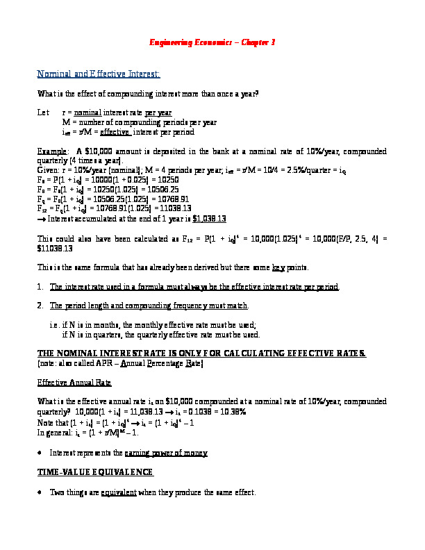
Nominal and Effective Interest:
What is the effect of compounding interest more than once a year?
Let r = nominal interest rate per year
M = number of compounding periods per year
ieff = r/M = effective interest per period
Example: A $10,000 amount is deposited in the bank at a nominal rate of 10%/year, compounded quarterly (4 times a year).
Given: r = 10%/year (nominal); M = 4 periods per year; ieff = r/M = 10/4 = 2.5%/quarter = iQ
F3 = P(1 + iQ) = 10000(1 + 0.025) = 10250
F6 = F3(1 + iQ) = 10250(1.025) = 10506.25
Fq = F6(1 + iQ) = 10506.25(1.025) = 10768.91
F12 = Fq(1 + iQ) = 10768.91(1.025) = 11038.13
Interest accumulated at the end of 1 year is $1,038.13
This could also have been calculated as F12 = P(1 + iQ)4 = 10,000(1.025)4 = 10,000(F/P, 2.5, 4) = $11038.13
This is the same formula that has already been derived but there some key points.
1. The interest rate used in a formula must always be the effective interest rate per period.
2. The period length and compounding frequency must match.
i.e. if N is in months, the monthly effective rate must be used;
if N is in quarters, the quarterly effective rate must be used.
THE NOMINAL INTEREST RATE IS ONLY FOR CALCULATING EFFECTIVE RATES.
(note: also called APR – Annual Percentage Rate)
Effective Annual Rate
What is the effective annual rate ia on $10,000 compounded at a nominal rate of 10%/year, compounded quarterly? 10,000(1 + ia) = 11,038.13 ia = 0.1038 = 10.38%
Note that (1 + ia) = (1 + iQ)4 ia = (1 + iQ)4 – 1
In general: ia = (1 + r/M)M – 1.
Interest represents the earning power of money
TIME-VALUE EQUIVALENCE
Two things are equivalent when they produce the same effect.
- effective interest rate computed for a nominally stated interest rate is an equivalent expression of the interest charge since both interest charges produce the same effect on an investment.
We differentiate between:
- Purchasing power of money: the amount of goods that can be purchased with a given sum of money. This varies up and down as a function of special localized circumstances and nationwide or worldwide economic conditions
- Earning power of money: this relates time and earnings to locate time-equivalent money amounts if $1000 were sealed and buried today, it would have a cash value of $1000 when it was dug up 2 years from now. Regardless of changes in buying power, the value remains constant because the earning power of the money was forfeited.
Consider $1000 deposited at 10% compounded annually. In two years, this amount will have a value of $1000(1 + 0.10)2 = $1210. Therefore, $1000 today is equivalent to $1210 in 2 years from now, if it earns interest at a prevailing rate of 10% compound yearly. Similarly, to have $1000 in 2 years from now, one needs only to deposit today.
If 10% is an acceptable rate of return, an investor will be indifferent between having $826.45 in hand or having a trusted promise to receive $1000 in 2 years.
Consider further that the $1000 could have been used to pay two equal annual $500 installments. The buried $1000 could be retrieved after 1 year, an installment paid, and the remaining $500 reburied until the second repayment became due.
If the $1000 is deposited at 10% instead, $1100 would be available at the end of the first year. After the first $500 installment was paid, the remaining $600 would draw interest until the next payment. Paying the second $500 installment would leave $600(1.1) - $500 = $160 in the account.
Because of the earning power of money, the initial deposit could have been reduced to $868.77 to pay out $500 at the end of each of the 2 years:
First year: $868(1.10) - $500 = $955 - $500 = $455 ($454.55)
Second year: $455(1.10) = $500 = second installment.
The $868 is equivalent to $500 received 1 year from now plus another $500 received 2 years from now:
First year: $500/1.10 = $455
Second year: $455 + $500/(1.10)2 = $455 + $413 = $868
The annual effective interest can be calculated from the effective interest rate per period.
Continuous Compounding
In the limit where M tends to infinity, compounding is every instant. This approach may be used for enormous transactions (between banks or countries) and also for theoretical models in economics.
effective interest in the case of continuous compounding is calculated by:
iC = er – 1 (where r is the nominal rate)
Example: If r = 18.232% compounded continuously what is iC?
iC = e0.18232 – 1 = 0.20 or 20%
Example: If iC = 22.1%, what is the nominal rate r?
0.221 = er – 1
1.221 = er ln (1.221) = r ln e
r = 0.20 or 20%
Example: Examine the effect of increased compounding frequency.
r(APR) = 10%; Discrete: ia = ; Continuous: iC = er - 1
Frequency
M
ia%
annual
1
10.00
semi-annual
2
10.250
quarterly
4
10.381
monthly
12
10.471
weekly
52
10.506
daily
365
10.515
continuous
10.517
PAYMENTS AND COMPOUNDING PERIODS MUST BE MADE COMPATIBLE BEFORE PERFORMING CALCULATIONS
Case (1): Payments less frequent than compounding
Example: Three deposits of $2500 will be made every 2 years, starting in 2 years. If i = 10%/year how much will be in the bank in 6 years?
The F/A formula cannot be applied directly because the cash flow frequency is not synchronized with the compounding periods. Solving one term at a time:
F = 2500 [(F/P, 10, 4) + (F/P, 10, 2) + 1] = 2500 [(1.4641) + 1.21 + 1] = $9,185
Alternatively, an equivalent effective interest rate per 2-year period can be found
ieff = (1.10) 2 –1 = 0.21 = 21%
F = 2500(F/A, 21, 3) = 2500(3.6741) = $9,185
Example: You have a loan requiring payments of $500 every 6 months for the next 2 years. Assume that the next payment is due tomorrow. The interest rate is 12% compounded monthly. If you wish to pay off the loan now, how much do you owe?
[Concept: PV of remaining payments is what you owe now, i.e. both you and the lender are indifferent between PV and rest of payments]
PV = 500 + 500(P/A, is, 4) an effective semi-annual rate is is needed.
The effective monthly rate is:
The effective semi-annual rate is: (1 + is) = (1 + im)6 is = (1.01)6 – 1 = 0.06152 s-a
PV = 500 + 500 (P/A, 0.06152, 4) = $2,226.54
Case (2): Payments more frequent than compounding
Example: Payments of $50 are made at the end of each month, APR = 12% compounded quarterly what is F at the end of 1 year?
2 APPROACHES depending on assumptions:
(a) All payments accumulate to the end of compounding period (i.e., they are not earning interest until then) In this case $150 accumulates every quarter F = 150 (F/A, 3, 4) = $627.54
(b) Calculate an effective interest rate per period 1 + iQ = (1 + im)3 im = (1.03)1/3 – 1 = 0.0099 F = 50 (F/A, 0.99, 12) = $633.79
The text assumes (b) unless otherwise stated
Varying Interest Rates
Must translate cash flows in stages, stopping at every boundary where the interest rate changes.
Example 1 P = $1000 F10 = ?
336804011747500153924011747500414528012509500473202012509500230886012509500480060117475005036820184150041224201079500228600010795004648201079500443484031758%
008%
306324031756%
006%
123444031754%
004%
3905251384300
000
497014513843010
0010
45205651384309
009
40690801403358
008
36118801403357
007
31470601403356
006
26974801403355
005
22402801403354
004
17678401479553
003
13030201479552
002
8382001479551
001
3200401479550027355804889500320802048895003657600488950041224204889500457200048895005036820488950022860004889500182118048895001371600488950090678048895004648204889500
F10 = 1000(1.04)4 (1.06)4 (1.08)2 = $1,722.68
What is the average 10-year yield?
(1 + i10)10 = (1.04)4 (1.06)4 (1.08)2 i10 = 5.589%
56769001638300048006001562108%
008%
38862001562106%
006%
32461201562105%
005%
429006016383000384048016383000750570017145000293370016383000Example 2 Find the equivalent annuity.
4175760876300038633409525000354330095250004312920876300050977808001000295656010287000720090010287000
4290060952500033756609525000567690010287000276606010287000567690026670005204460266700047548802667000429006026670003840480266700033756602667000293370026670002867025704850
000
5623560723906
006
5173980723905
005
4716780723904
004
4244340800103
003
3779520800102
002
3314700800101
001
3177540-26670600
00600
411480057150700
00700
5440680952501,000
001,000
600 (P/F, 5, 1) + 700 (P/F, 6, 1)(P/F, 5, 2) + 1000 (P/F, 7, 3)(P/F, 6, 1)(P/F, 5, 2)
= A[(P/A, 5, 2) + (P/F, 6, 1)(P/F, 5, 2) + (P/A, 7, 3)(P/F, 6, 1)(P/F, 5, 4)
A = $472.47
CRITERIA FOR EVALUATING OPTIONS
Justification for choice of criteria
Cash flows which occur at different points in time cannot be directly compared an equivalent amount at some point in time, such as a present value to combine cash flows, has to be calculated.
- Several criteria are available to evaluate a proposal. The main ones are:
Present Worth (PW) – (Chapter 4)
Future Worth (FW) – (Chapter 4)
Annual Worth (AW) – (Chapter 5)
Internal Rate of Return (IRR) – (Chapter 6)
- A particular criterion might be the best one for a certain situation while in other situations, a combination of several criteria may be appropriate.
- The use of the Present Worth analysis is the easiest and most common approach but other criteria also provided useful information.
SOME USEFUL CONCEPTS
Minimum Acceptable (Attractive) Rate of Return (MARR)
Every company or individual must select a suitable interest rate to evaluate the time value of money. Most companies establish a minimum acceptable (attractive) rate of return (MARR) for internal calculations. It is affected by many factors, such as:
- prevailing market (i.e., bank) rates
- cost of capital
- risk of business
- historical rates earned in the company
Example: A company ("JIVE-T" in Halifax is considering buying a new machine for bagging their chips. One possible model costs $120,000 with an estimated salvage value of $5,000 at the end of a ten year useful life. Given the anticipated growth in sales, the expected savings are $15,000 in the first year, increasing by $5,000 in subsequent years. Operating costs are $10,000/year. The MARR is 12%.
4983480-60960$5,000 - salvage
00$5,000 - salvage
914400762000050292006858000456438016002000
208788099060G = $5,000/year
00G = $5,000/year
41148007620000364998016764000
31927808382000
388620213360$15,000
00$15,000
497586022860$60,000
00$60,000
273558000022707609144000
1821180762000136398010668000
906780152400045720012954000
4960620010
0010
320040457200039624000
000
242316091440-$10,000
00-$10,000
90678012192000
396240243840-$120,000
00-$120,000
Project Screening
Certain simple techniques can be used to ascertain whether a project is viable, before detailed analysis is done. Since uncertainty increases tremendously the further into the future we go, one common requirement is that an investment generates enough revenues to cover the initial cost within a reasonable time frame. The criterion is called the payback period.
Payback Period
(a) Without interest (faster, but inaccurate) Given Ft, the cash flow in period t, the payback period corresponds to the smallest value of n for which:
(b) With interest (discounted payback period) the payback period requires that the PV (Present Value) of revenues surpass the PV of expenses. Therefore, the smallest value of n which satisfies: is the payback period.
Example: "JIVE-T" payback:
Without interest
With interest
N
Outflows
Inflows
Net flow
Sum (t = 0 ton)
PV(t = 0 ton)
0
$(120,000)
0
$(120,000)
$(120,000)
$(120,000)
1
$(10,000)
$15,000
$5,000
$(115,000)
$(115,535)
2
$(10,000)
$20,000
$10,000
$(105,000)
$(107,564)
3
$(10,000)
$25,000
$15,000
$(90,000)
$(96,887)
4
$(10,000)
$30,000
$20,000
$(70,000)
$(84,177)
5
$(10,000)
$35,000
$25,000
$(45,000)
$(69,991)
6
$(10,000)
$40,000
$30,000
$(15,000)
$(54,722)
7
$(10,000)
$45,000
$35,000
$20,000
$(38,960)
8
$(10,000)
$50,000
$40,000
$60,000
$(22,805)
9
$(10,000)
$55,000
$45,000
$105,000
$(6,577)
10
$(10,000)
$65,000
$55,000
$160,000
$11,131
Therefore, using the undiscounted method suggests that the investment begins paying back after year 6, whereas if discounting is included, it isn't until year 10 that the project becomes viable.
Drawbacks to the Payback Period Method
An important limitation of this method is that it does not account for cash flows occurring after the payback period. For example, assume that in year 11 of the "JIVE-T" example, there is an overhaul cost of $100,000 and then revenues are constant. Overall, the project would not be viable. Because of this deficiency, the method should not be used as the sole decision-making criterion.
PRESENT VALUE
To see if the "JIVE-T" project is a good investment
5387340-5334000
4062095-69850002621915-6985000PV = -$120,000 + [$15,000 + $15,000(A/G, 12, 10) - $10,000](P/A, 12, 10) + $5,000(P/F, 12, 10)
(3.5847) (5.6502) (0.3222)
PV = $11,132
Conclusion: Since the PV is greater than zero, the project is economical. Note that even if PV = 0 exactly, we accept the project, because the investment returns 12%. The fact that PV > 0 shows that they make a surplus above 12%.
INVESTMENT POOL CONCEPT: to explain the meaning of PW > 0
assumption: funds not used in this project can earn MARR elsewhere in the company
Example: $120,000 would be worth FV(@12%) = $372,702 in 10 years if NOT invested in "JIVE-T". If instead the $120,000 WERE invested in "JIVE-T", then the FV(@MARR) of the net cash flows for the 10 years ($120,000 + $11,132)(1.12)10 = $407,276. Therefore investing in "JIVE-T" earns us an additional $34,574 by year 10. The present value of this amount is $11,132! Therefore, once can see that a positive PV indicates a gain over and above the MARR.
CONDITIONS FOR PRESENT-WORTH COMPARISONS
Cash flows are known.
Cash flows are in constant-value dollars.
The interest rate is known.
Comparisons are made with before-tax cash flows.
Comparisons do not include intangible considerations.
Comparisons do not include consideration of the availability of funds to implement alternatives.
EQUIVALENT ANNUAL WORTH (AW)
3284855-69215005235575-75565001296035-6794500AW = $120,000(A/P, 12, 10) + $15,000 = $5,000(A/G, 12, 10) - $10,000 + $5,000(A/F, 12, 10)
(0.1770) (3.5847) (0.0570)
AW = $1968/year
Naturally, this same result is obtained directly by starting with the present value
AW = PV(A/P, 12, 10) = $11,132(0.1770) = $1970
It is evident that the AW is positive if the PV is positive and vice versa. If one is negative, the other is also negative. Therefore, the two criteria always give consistent results.
FUTURE VALUE
The same reasoning applies when the future value criterion is used. FV is also a consistent measure of project viability because it differs from the PV (or AW) by a positive constant.
Note:
INTERNAL RATE OF RETURN (IRR)
Given all of the foreseen cash flows and their occurrence, we can calculate the only unknown for which the PV (or FW or AW) equals zero, i. The value of i, if it exists gives the effective interest earned (or charged) on money. That is, if I lend $100 for a month and demand a reimbursement of $150 at the end of the month, the internal rate of return is 50% per month.
PV = $100 = FV(P/V, i, 1) = $150(P/F, i, 1) = ($150) (1 + i)1 = = 1.5 i = 0.5 = 50%
The same reasoning applies for a more complicated set of transactions. For example examining the "JIVET" problem, the IRR can be calculated by solving for:
PV = 0 = -$120,000[$15,000 + $5,000(A/G, i, 10) - $10,000](P/A, i, 10) + $5,000(P/F, i, 10)
Solving the non-linear equation for the unknown i by trial and error, or using software such as Excel, we find i = 13.6%.
Conclusion: Since the MARR = 12%, this project is viable because IRR > MARR.
CAUTION: We would expect all of these methods to lead to the same conclusion. However, difficulties can arise because of the non-linear nature of the PV equation when solving for i (i.e, multiple roots). This difficulty will be considered shortly.
PW PROFILE (see also Figure 4.19, p. 24 Text)
315468041148000To better understand the meaning of the IRR, consider the PW of the cash flow series as a function of i. Two points are easy to place to place on the graph: the IRR is the horizontal intercept (by definition); and the PV (@ i = 0) is the sum of the cash flows. Note what happens as i ?. The curve asymptotically approaches the initial cash flow at time zero! Why?
We can see that since the IRR > MARR, the project is acceptable. As long as this PW profile applies to the problem at hand, the IRR criteria and PW criteria lead to the same conclusion in a straight-forward manner. Exceptions to this will be reviewed later.
We also see that the PW > 0 at MARR, as expected.
Hints to save time when calculating IRR by trial and error
1. Identify the most important elements in a complicated calculations, and estimate an initial approximate interest rate based on these values.
2. Add the receipts and expenses without discounting (i.e., i = 0). If the sum is negative the IRR is less than zero (for an investment type of analysis). If the sum is positive, its value may suggest a reasonable guess for IRR to start.
3. If the salvage value is close to the initial cost, and there is an annuity, A/P = i.
4. The rule of 72: a sum doubles in value about every 72/i years.
5. Since interest rates are often less than 25%, an initial guess of 10% is reasonable.
6. Obviously, a financial calculator or spreadsheet is best.
Rule of 72:
This is a handy rule-of-thumb which provides a useful approximation to the time required to double money: n = 72/i.
Where does this rule come from? Starting with the formula for (F/P, i, n): F = P(1 + i)n
To double money (F = 2P): 2P = P(1 + i)n Simplifying: 2 = (1 + i)n
ln(2) = n ln(1 + i) n = ln(2)/ln(1 + i)
ln(2) = 0.6931 and ln(1 + i) i for small i (see graph) n 0.72/i = 72/i %
Note: 72 gives a better approximation than 70.
Example 1:
(a) If we deposit $1,000 in the bank at 7% for 10 years: P = $1,000, i = 7%, n = 10, F = P(F/P, 7, 10) = 1,000(1.96715) = $1967.15.
(b) How much must we put in the bank now at 9%/year to accumulate $5,000 in 8 years? F = $5,000, i = 9%, n = 8, P = F(P/F, 9, 8) = $5,000(0.5019) = $2,509,39
Example 2:
N = 5 years, P = $80,000, F = $150,000
revenue: $1,500/year (= A+)
expenses: $850/year (= A-)
5296535-7112000To find i: P = F(P/F, i, N) + (A+-A-)(P/A, i, N) $80,000 = $150,000(P/F, i, 5) + $(1,500 – 850)(P/A, i, 5)
$650
Using the rule of 72:
Since $150,000 is almost the double of $80,000, if we ignore the annuity, we get i 14.4% ( = 72/5). So use initial estimate of i = 14%.
2902585-41910001764030-3873500 $150,000(P/F, 14, 5) + $650(P/A, 14, 5) = $80,136
0.51937 3.433
Since the results is greater than $80,000, we try a higher rate (to reduce the PV of the future transactions). So for i = 15%:
2903220-53340001764030-2857500 $150,000(P/F, 15, 5) + $650(P/A, 15, 5) = $76,756
0.4972 3.3522