Transcript
Table of Contents
Introduction 3
Theoretical Background 4
Experimental/Simulation Procedure 2
Process Flowsheet: 2
Dynamic Simulation 2
Results and Discussion 4
Error Analysis 6
Conclusion and Recommendations 6
References 6
Appendices 6
Raw Data 6
Sample Calculations 6
Introduction
Aspen HYSYS is an easy-to-use process modeling environment that enables optimization of conceptual design and operations Aspen HYSYS is used for simulations of processes to act upon situations in a real manner. Designing processes or setting parameters is costly due to downtime or capital costs. HYSYS is used to simulate a run-through without a negative impact. It is more efficient to predict certain situations therefore allowing for engineers to tweak and alter parameters.
The objective of this lab is to compare the functionalities between Proportional (P), Proportional integral (PI) and proportional integral derivative (PID) controllers. In this experiment, a process will be created through HYSIS and controlled by the use of PID controllers in a separation unit. PID controller is a control loop feedback mechanism widely used industrial control systems. A PID controller calculates an error value as the difference between a measured process variable and a desired set point. The controller attempts to minimize the error by adjusting the process through use of a manipulated variable. The PID controller in this experiment is used to control pressure and liquid level %. The inputs that are used to control the system are the target set points, as well as the maximum and minimum values to ensure the process does not overshoot or undershoot the system. With the use of dynamic simulations, as well as strip charts and controller tuning, control systems will be identified and a better understanding of PID controllers will be established.
Theoretical Background
The purpose of a process control systems is ensure steady-state operations, process stability, high productivity, safety, and process optimization since most processes are multivariable and interactive. There are different two controller types used in the industry; feed-backward and feed-forward. In this experiment, the designed controller is feed-backward dependent. A PID (Proportional-integral-derivative controller), a type of a feed-back controller, is used to show the effects of changes on the control parameters. In dynamic mode, the simulation allows for thermodynamic properties to be approximated using polynomial interpolation in the vicinity of the operating point, rather than more accurate estimates that are more time consuming to compute. Once the PID controller is selected and placed onto the PFD, a Process variable (PV) is controlled and defined as:
PV%=PV-PVminPVmax-PVmin*100
(1)
(Dhib,2012)
The controller output (OP) is manipulated by the controller according to the percentage of its set limit. In this case, taking into the account the tuning parameters Kc, ?i, and ?d, the output function of a PID can be represented by the mathematical equation:
OPt=OPss+Kc[Et+1?i·0tE?d?+?ddEtdt]
(2)
(Dhib,2012)
Where
Opss = bias (controller output at zero error)
Kc= proportional gain
?I = integral time constant
?d = derivative time constant
Experimental/Simulation Procedure
Process Flowsheet:
HYSIS program was opened, Fluid package was started (Peng Robinson) and gas stream components with the following composition:
Methane = 0.35
Ethane =0.25
n-ethane =0.10
Propane =0.10
I-butane =0.10
I-pentane =0.05
n-pentane = 0.03
n-hexane = 0.02
Feed parameters were added with T=60°F, P=850psia and molar flow rate at 1000 lbmole/hr
Separator was added to the flow sheet with all inlet and outlet streams identified and parameters inputted
2 PID controllers were added to both vapour and liquid streams and a specified properties were inputted. Controller name for Liquid is Sep-LLC and controller name for vapour was Sep-PC.
Sep-LLC: PVmin = 0 and PVmax = 100
Sep-PC: PVmin = 500 and PVmax = 1000
3 Strip Charts were added, edited and named Vessel Pressure, Liquid Level Percent, and Liquid mass flow.
File was saved as a Steady-system
Dynamic Simulation
Entered Dynamic Mode
Clicked Integrator to set run time of system for 30 minutes
Saved file as a Dynamic System
First case: Proportional controller (P) set point @ 60% and tuning of proportional gain, Kc=1 and dynamic system was run. Strip Charts were displayed and analyzed
Second Case: Proportional integrator set point at 60% and tuning of proportional gain, Kc=1, integral time constant ?i=0.02 and dynamic system was run. Strip Charts were displayed and analyzed
Third case: Proportional integrator set point at 60% and tuning of proportional gain, Kc=1, integral time constant ?i=0.02, derivative time constant ?d=10, 1, 0.1, 0.01 was used and dynamic system was run. Strip Charts were displayed and analyzed
Figure 1 Steady-state Flow sheet of overall System
Figure 2 Dynamic Flow-sheet of overall system
Results and Discussion
Figure 3: Vapour Pressure with : Ki=1, ?i= empty , ?d= empty
Figure 4 Vapour Pressure with : Ki=1, ?i= 0.02 , ?d= empty
Figure 4: Liquid Level Percent with : Ki=1, ?i= empty , ?d= empty
Figure 5 Liquid Mass Percent with : Ki=1, ?i= empty , ?d= empty
Case 2: Ki=1, ?i= 0.02, ?d= empty
Figure 7: Liquid Level Percent with : Ki=1, ?i= 0.02 , ?d= empty
Figure 8: Liquid Mass Percent with : Ki=1, ?i= 0.02 , ?d= empty
Case 3 Part a : Ki=1, ?i= 0.02, ?d= 10
Figure 9: Vapour Pressure with : Ki=1, ?i=0.02, ?d= 10
Figure 10: Liquid Level Percent with : Ki=1, ?i= 0.02 , ?d= 10
Figure 11: Liquid Mass Percent with : Ki=1, ?i= 0.02 , ?d= 10
Case 3 Part b : Ki=1, ?i= 0.02, ?d= 0.01
Figure 12: Vapour Pressure with : Ki=1, ?i= 0.02 , ?d= 0.01
Figure 13: Liquid Level Percent with : Ki=1, ?i= 0.02 , ?d=0.01
Figure 14: Liquid Mass Percent with : Ki=1, ?i= 0.02 , ?d= 0.01
Error Analysis
Conclusion and Recommendations
References
Dhib, R. (Fall 2012B). Process Control Laboratory Manual. Toronto: Ryerson University.
Perry, H.H., and D. Green, Perry’s Chemical Engineers’ Handbook, 6th Ed., McGraw-Hill Inc., New York, 1984
Nasri, Z., & Binous, H. (2009). Applications of the Peng-Robinson Equation of State using MATLAB.43(2). Retrieved from http://cache.org/site/news_stand/summer09/summer09 Binous applic of equation.pdf
Seader, J.D. and E.J. Henley, Separation Process Principles, John Wiley & Sons, 1998
Appendices
Raw Data
Sample Calculations